https://ift.tt/efpnT5c Make stronger and simpler models by leveraging natural order Co-authored with Dmytro Karabash Photo by JD Rincs ...
Make stronger and simpler models by leveraging natural order
Co-authored with Dmytro Karabash

Introduction
Imagine that you have 2,000 features and you need to make the best predictive model (“best” in terms of complexity, interpretation, compliance, and — last but not least — performance). Such a case will be familiar to anyone who has ever worked with a large set of categorical variables and employed the popular One-hot encoding method. Usually, sparse data sets don’t work well with highly efficient tree-based algorithms like Random Forest or Gradient Boosting.
Instead, we recommend finding an ordinal encoding, even when there is no obvious order in categories. We introduce the Rainbow method — a set of techniques for identifying a good ordinal encoding — and show that it has multiple advantages over the conventional One-hot when used with tree-based algorithms.
Here are some benefits of the Rainbow method compared to One-hot:
- Resource Efficiency
- Saves substantial modeling time
- Saves storage
- Notably reduces computational complexity
- Reduces or removes the need for “big data” tools such as distributed processing
2. Model Efficiency
- Significantly reduces model dimensionality
- Preserves data granularity
- Prevents overfitting
- Models reach peak performance with simpler hyperparameters
- Naturally promotes feature selection
Background
Data scientists with different backgrounds might have varying favorite approaches to categorical variables encoding. The general consensus, though, is that:
- Categorical variables with a natural ordering should use encoding that respects that ordering, such as ordinal encoding; and
- Categorical variables without a natural ordering — i.e. nominal variables — should use some kind of nominal encoding, and One-hot is the most commonly-used method.
While One-hot encoding is often employed reflexively, it can also cause multiple issues. Depending on the number of categories, it can create huge dimensionality increase, multicollinearity, overfitting, and an overall very complex model. These implications contradict Occam’s Razor principle.
It is neither often nor generally accepted when modelers apply ordinal encoding to a categorical variable with no inherent order. However, some modelers do it purely for modeling performance reasons. We decided to explore (both theoretically and empirically) whether such an approach provides any advantages, as we believe that encoding of categorical variables deserves a deeper look.
In fact, most of the categorical variables have some order. The two examples above — a perfect natural ordering and no natural ordering — are just the extreme cases. Many real categorical variables are somewhere in between. Thus, turning them into a numeric variable would be neither exactly fair nor exactly artificial. It would be some mix of the two.
Our main conclusion is that ordinal encoding is likely better than One-hot for any categorical variable, when used with tree-based algorithms. Moreover, the Rainbow method we introduce below helps select an ordinal encoding that makes the best logical and empirical sense. The Rainbow method also aspires to support interpretability and compliance, which are important secondary considerations.
Linear vs. Tree-based Models
Formal statistical science separates strictly between quantitative and categorical variables. Researchers apply different approaches to describe these variables and treat them differently in linear models, such as Regression. Even when certain categorical variables have natural ordering, one should be very cautious about applying any quantitative methods to them.
For example, if the task is to build a linear model where one independent variable is Education Level, then the standard approach is to encode it via One-hot. Alternatively, one could engineer a new quantitative feature Years of Education to replace the original variable — although in that case, it would not be a perfectly equivalent replacement.
Unlike linear models, tree-based models rely on variable ranks rather than exact values. So, using ordinal encoding for Education Level is perfectly equivalent to One-hot. It would actually be overkill to use One-hot for variables with clear natural ordering.
In addition, the values assigned to categories won’t even matter, so long as the correct order is preserved. Take, for example, Decision Trees, Random Forest, and Gradient Boosting — each of these algorithms will output the same result if, say, the variable Number of Children is coded as
0 = “0 Children”
1 = “1 Child”
2 = “2 Children”
3 = “3 Children”
4 = “4 or more Children”
or as
1 = “0 Children”
2 = “1 Child”
3 = “2 Children”
4 = “3 Children”
5 = “4 or more Children”
or even as
-100 = “0 Children”
-85 = “1 Child”
0 = “2 Children”
10 = “3 Children”
44 = “4 or more Children”
The values themselves don’t serve a quantitative function in these algorithms. It is the rank of the variable that matters, and a tree-based algorithm will use its magic to make the most appropriate splits for introducing new tree nodes.
Decision trees don’t work well with a large number of binary variables. The splitting process is not efficient, especially when the fitting is heavily regularized or constrained. Because of that, even if we randomly order categories and make a single label encoded feature, it would still likely be better than One-hot.
Random Forest and Gradient Boosting are often picked among other algorithms due to better performance, so our method could prove handy in many cases. The application of our method to other algorithms, such as Linear Regression or Logistic Regression, is out of the scope of this article. We expect that this method of feature engineering may still be beneficial, but that is subject to additional investigation.
Method
Think of a clearly nominal categorical variable. One example is Color. Say, the labels are: “Green”, “Red”, “Blue”, “Violet”, “Orange”, “Yellow”, and “Indigo”.
We would like to find an order in these labels, and such an order exists — a rainbow. So, instead of making seven One-hot features, you can simply create a single feature with encoding:
0 = “Red”
1 = “Orange”
2 = “Yellow”
3 = “Green”
4 = “Blue”
5 = “Indigo”
6 = “Violet”
Hence, we called the set of techniques to find an order in categories the “Rainbow method”. We found it amazing that there exists a natural phenomenon that represents label encoding for a nominal variable!
Generalizing this logic, we suggest finding a rainbow for any categorical variable. Even if possible ordering is not obvious, or if there doesn’t seem to be one, we offer some techniques to find it. Oftentimes, some order in categories exists, but is not visible to the modelers. It can be shown that if the data-generating process indeed presumes some order in categories, then utilizing it in the model will be substantially more efficient than splitting categories into One-hot features. Hence our motto:
“When nature gives you a rainbow, take it…”
According to our findings, the more clearly defined the category order, the higher the benefits in terms of model performance for using ordinal encoding instead of One-hot. However, even in the complete absence of order, making and using random Rainbow is likely to result in the same model performance as One-hot, while saving substantial dimensionality. This is why searching for a rainbow is a worthwhile pursuit.
Is Color a nominal variable?
Some readers might argue that Color is clearly an ordinal variable, so it is no surprise that we found an ordinal encoding.
On the one hand, modelers from different scientific backgrounds may view the same categorical variables differently and are probably used to applying certain encoding methods reflexively. For example, I (Anna) studied Economics and Econometrics, and I did not encounter any use case that could treat Color as quantitative. At the same time, modelers that studied Physics or Math might have utilized wavelength in their modeling experience, and likely considered Color ordinal. If you represent the latter modelers, please take a minute and think of a different example of a clearly nominal variable.
On the other hand, whether natural ordering exists or not does not change our message. In short, if the order exists — great! If it does not… well, we want you to find it! We will provide more examples below and hope they can guide you on how to find a rainbow for your own example nominal variable.
At first glance, most nominal variables seem like they cannot be converted to a quantitative scale. This is where we suggest finding a rainbow. With color, the natural scale might be hue, but that’s not the only option — there’s also brightness, saturation, temperature, etc. We invite you to experiment with a few different Rainbows that might capture different nuances of the categorical quality.
You can actually make and use two or more Rainbows out of one categorical variable, depending on the number of categories K and the context.
We don’t recommend using more than log₂(K) Rainbows, because we do not want to surpass the number of encodings in a Binary One-hot.
The Rainbow method is very simple and intuitively sensible. In many cases, it is not even that important which Rainbow you choose (and by that, we mean the color order); it would still be better than One-hot. The more natural orders are just likely to perform better than others and be easier to interpret.
Finding a Rainbow — Examples
The statistical concept of level of measurement plays an important role in separating variables with natural ordering from the variables without it. While quantitative variables have a ratio scale — i.e. they have a meaningful 0, ordered values, and equal distances between values — categorical variables have either interval, ordinal, or nominal scales. Let us illustrate our method for each of these types of categorical variables.
Interval variables have ordered values and equal distances between values, but the values themselves are not necessarily meaningful. For example, 0 does not indicate the absence of some quality. Common examples of interval variables are Likert scales:
How likely is the person to buy a smartphone?
1: “Very Unlikely”
2: “Somewhat Unlikely”
3: “Neither Likely Nor Unlikely”
4: “Somewhat Likely”
5: “Very Likely”
Without a doubt, interval variables intrinsically give us the best and most natural Rainbow. Most modelers would encode them numerically.
1 = “Very Unlikely”
2 = “Somewhat Unlikely”
3 = “Neither Likely Nor Unlikely”
4 = “Somewhat Likely”
5 = “Very Likely”
Notation: we use a “colon” sign to denote raw category names and an “equals” sign to denote assignment of numeric values to categories.
Ordinal variables have ordered meaningless values, and the distances between values are neither equal nor explainable.
What is the highest level of Education completed by the person?
A: “Bachelor’s Degree”
B: “Master’s Degree”
C: “Doctoral Degree”
D: “Associate Degree”
E: “High School”
F: “No High School”
Similar to interval variables, ordinal variables have an inherent natural Rainbow. Sometimes, the categories for an ordinal variable are not listed according to the correct order, and that might steer us away from seeing an immediate Rainbow. With some attention to the variables, we could reorder categories and then use this updated variable as a quantitative feature.
1 = “No High School”
2 = “High School”
3 = “Associate Degree”
4 = “Bachelor’s Degree”
5 = “Master’s Degree”
6 = “Doctoral Degree”
So far, most modelers would organically use the best Rainbow. The more complicated question is how to treat nominal variables.
Nominal variables have no obvious order between categories. The intricacy is that for machine learning modeling goals, we could be more flexible with variables and engineer features, even if they make little sense from a statistical standpoint. In this way, using Rainbow method, we can turn a nominal variable into a quantitative one.
The main idea behind finding a rainbow is the utilization of either human intelligence or automated tools. For relatively small projects where you can directly examine every categorical variable, we recommend putting direct human intelligence into such a selection. For large-scale projects with many complex data sets, we offer some automated tools to generate viable quantitative scales.
Manual Rainbow Selection
Let’s look at some examples of manual subjective Rainbow selection. The trick is to find a quantitative scale by either using some concrete related attribute or constructing that scale from a possibly abstract concept.
In our classical example, for a nominal variable Color, the Hue attribute suggests a possible scale. So, the nominal categories
A: “Red”
B: “Blue”
C: “Green”
D: “Yellow”
can be replaced by the newly-engineered Rainbow feature:
1 = “Blue”
2 = “Green”
3 = “Yellow”
4 = “Red”
For the Vehicle Type variable below,
Vehicle Type
C: “Compact Car”
F: “Full-size Car”
L: “Luxury Car”
M: “Mid-Size Car”
P: “Pickup Truck”
S: “Sports Car”
U: “SUV”
V: “Van”
we can think of dozens of characteristics to make a Rainbow — vehicle size, capacity, price category, average speed, fuel economy, costs of ownership, motor features, etc. Which one (or a few) to pick? The choice depends on the context of the model. Think about how this feature can help predict your outcome variable. You can try a few possible Rainbows and then choose the best in terms of model performance and interpretation.
Consider another variable:
Marital Status
A: “Married”
B: “Single”
C: “Inferred Married”
D: “Inferred Single”
This is where we can get a bit creative. If we think about Single and Married as being two ends of a spectrum, then Inferred Single could be between the two ends, closer to Single, while Inferred Married would be between the two ends, closer to Married. That would make sense because Inferred holds a certain degree of uncertainty. Thus, the following order would be reasonable:
1 = “Single”
2 = “Inferred Single”
3 = “Inferred Married”
4 = “Married”
In case there are any missing values, a new category, “Unknown”, fits exactly in the middle between Single and Married, as there is no reason to prefer one end to the other. Thus, the modified scale could look like this:
1 = “Single”
2 = “Inferred Single”
3 = “Unknown”
4 = “Inferred Married”
5 = “Married”
Another example:
Occupation
1: “Professional/Technical”
2: “Administration/Managerial”
3: “Sales/Service”
4: “Clerical/White Collar”
5: “Craftsman/Blue Collar”
6: “Student”
7: “Homemaker”
8: “Retired”
9: “Farmer”
A: “Military”
B: “Religious”
C: “Self Employed”
D: “Other”
Finding a rainbow in this example might be harder, but here are a few ways to do it: we could order occupations by average annual salary, by their prevalence in the geographic area of interest, or by information from some other data set. That might involve calling a Census API or some other data source, and could be complicated by the fact that these values are not static, but these are still viable solutions.
Automated Rainbow Selection
What if there is no good related attribute? In some situations, we cannot find a logical order for the Rainbow because the variable itself is not interpretable. Alternatively, what if we have very large data and no resources to manually examine each variable? This next technique is handy for such cases.
Let’s look at a black box column made by a third party:
Financial Cluster of the Household
1: “Market Watchers”
2: “Conservative Wealth”
3: “Specific Savers”
4: “Tried and True”
5: “Trendy Inclinations”
6: “Current Consumers”
7: “Rural Trust”
8: “City Spotlight”
9: “Career Conscious”
10: “Digital Financiers”
11: “Financial Futures”
12: “Stable Influentials”
13: “Conservatively Rural”
In this example, we have no clear idea of what each category entails, and therefore have no intuition on how to order these categories. What to do in such situations? We recommend creating an artificial Rainbow by looking at how each category is related to the target variable.
The simplest solution is to place categories in order of correlation with the target variable. So, the category with the highest value of correlation with the dependent variable would acquire numeric code 1, while the category with the lowest correlation would acquire numeric code 13. In this case, then, our Rainbow would mean the relationship between the financial cluster and the target variable. This method would work for both classification and regression models, as it can be applied to a discrete and a continuous target variable.
Alternatively, you can construct your Rainbows by merely utilizing certain statistical qualities of the categorical variable and the target variable.
For instance, in the case of a binary target variable, we could look at the proportion of ones given each of the categories. Suppose that among Market Watchers, the percentage of positive targets is 0.67, while for Conservative Wealth it is 0.45. In that case, Market Watchers will be ordered higher than Conservative Wealth (or lower, if the target percent scale is ascending). In other words, this Rainbow would reflect the prevalence of positive targets inside each category.
One reasonable concern with these automated methods is a potential overfit. When we use posterior knowledge of correlation or target percent that relates an independent variable with the dependent variable, this can likely cause data leakage. To tackle this problem, we recommend learning Rainbow orders on a random holdout sample.
Rainbow Preserves Full Data Signal
In this section, we briefly show that Rainbow ordinal encoding is perfectly equivalent to One-hot when used on decision trees. In other words, that full data signal is preserved.
We also show below that if the selected Rainbow (order of categories) agrees with the “true” one — i.e. with the data-generating process — then the resulting model will be strictly better than the One-hot model. To measure model quality, we will look at the number of splits in a tree. Less splits mean a simpler, more efficient and less overfit model.
Let us zoom in for a minute on a classical Rainbow example with only 4 values:
Color
0 = “Red”
1 = “Yellow”
2 = “Green”
3 = “Blue”
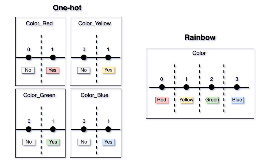
In the case of One-hot, we would create 4 features:
Color_Red = 1 if Color = 0 and 0 otherwise,
Color_Yellow = 1 if Color = 1 and 0 otherwise,
Color_Green = 1 if Color = 2 and 0 otherwise,
Color_Blue = 1 if Color = 3 and 0 otherwise.
In the case of Rainbow, we would just use Color by itself.
Let’s compare the possible models made using these two methods: 4 features vs. 1 feature. For simplicity’s sake, let’s build a single decision tree. Consider a few scenarios of the data-generating process.
Scenario 1
Assume that all the categories are wildly different and each one introduces a substantial gain to the model. This means that each One-hot feature is indeed critical — the model should separate between all 4 groups created by One-hot.
In that case, an algorithm like XGBoost will simply make the splits between all the values, which is perfectly equivalent to One-hot. There are exactly three splits in both models. Thus, the same exact result is achieved with just one feature instead of four.
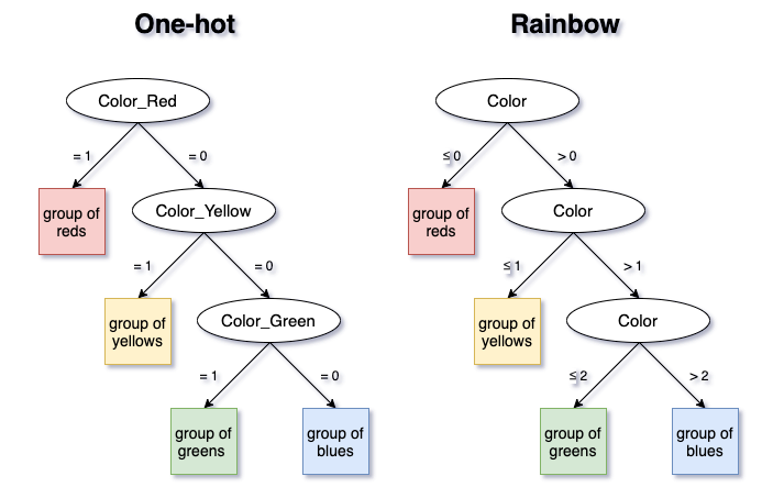
One can clearly see that this example is easily generalized to One-hot with any number of categories. Also, note that the order of the categories in Rainbow does not matter, as splits will be made between all categories. In practice, (K-1) splits will be sufficient for both methods to separate between K categories.
The main takeaway is that not a bit of data signal is lost when one switches from One-hot to Rainbow. Additionally, depending on the number of categories, a substantial dimensionality reduction happens, which saves time and storage, as well as reduces model complexity.
Sometimes, modelers try to beat One-hot’s dimensionality issue by combining categories into some logical groups and turning these into binary variables. The shortcoming of this method is its loss of data granularity. Note that by using Rainbow method, we do not lose any level of granularity.
Scenario 2
Let’s look at a less favorable scenario for Rainbow, where the chosen order does not agree with the “true” one. Let’s say that the data-generating process separates between the group of {Red, Green} and {Yellow, Blue}.
In this case, the algorithm will make all the necessary splits — three for Rainbow and two or three for One-hot, depending on the order of One-hot features picked up by the tree.
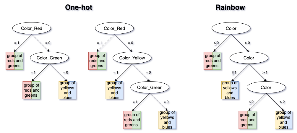
Even in this least favorable scenario, no data information is lost when choosing Rainbow method, because a tree with a maximum of (K-1) splits will reflect any data-generating process.
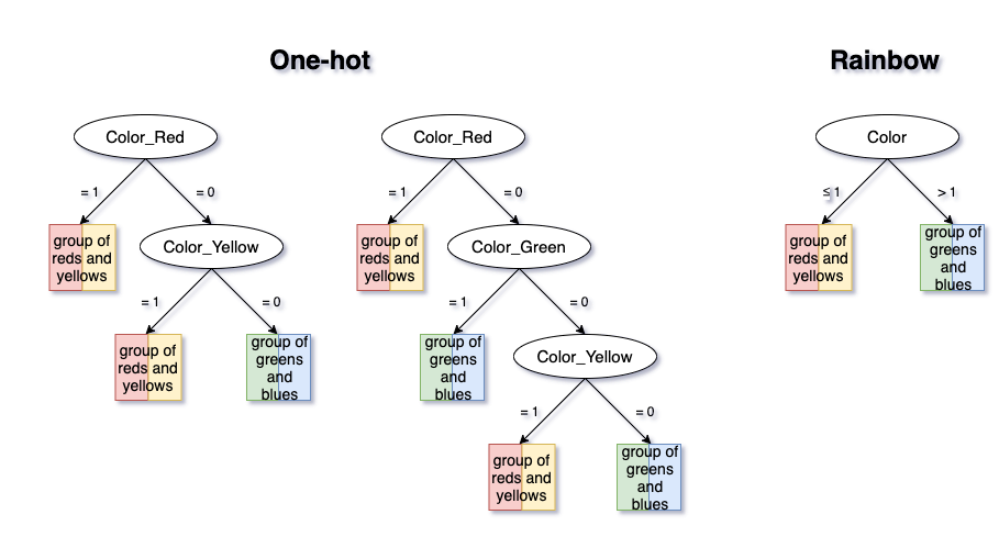
Scenario 3
Finally, if the data-generating process is actually in agreement with the Rainbow order, then the Rainbow method will be superior to One-hot. Not only will it not lose any data signal, it will also substantially reduce complexity, decrease dimensionality, and help avoid overfitting.
Suppose the true model pattern only separates between {Red, Yellow} and {Green, Blue}. Rainbow has a clear advantage in this case, as it exploits these groupings, while One-hot does not. While the One-hot model must make two or three splits, the Rainbow model only needs one.
Credits
We would like to cordially thank MassMutual’s Dan Garant, Paul Shearer, Xiangdong Gu, Haimao Zhan, Pasha Khromov, Sean D’Angelo, Gina Beardslee, Kaileen Copella, Alex Baldenko, and Andy Reagan for providing highly valuable feedback.
Original Idea by Dmytro Karabash
Hidden Data Science Gem: Rainbow Method for Label Encoding was originally published in Towards Data Science on Medium, where people are continuing the conversation by highlighting and responding to this story.
from Towards Data Science - Medium
https://towardsdatascience.com/hidden-data-science-gem-rainbow-method-for-label-encoding-dfd69f4711e1?source=rss----7f60cf5620c9---4
via RiYo Analytics


No comments