https://ift.tt/dV74H2D Plus a Data Insight Image by author. Table of Contents — Introduction — Signal Statistics — Get Bispectru...
Plus a Data Insight
Table of Contents
— Introduction
— Signal Statistics
— Get Bispectrum Images
— Load Images
— Create Model
— Train and Evaluate
— Loss and Accuracy Metrics
— Data Insight
— Conclusion
Introduction
Transfer learning reuses a model built for an old task as the starting point for a new task. Model parameters are frozen— training on the old task is done. VGG16 is one such trained model. It is a convolutional neural network (CNN) which classifies images. It won the 2014 ImageNet Challenge.
We slightly modify VGG16 to make it an effective classifier of new images. Model reuse greatly lowers training time and cost. This is the magic of transfer learning.
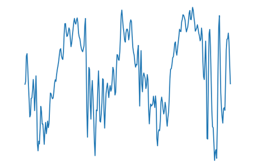
Our dataset is images produced from a 1-dimensional signal. A 1-dimensional signal is a sideways squiggly line. The signal amplitude moves up and down over time.
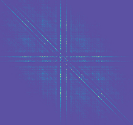
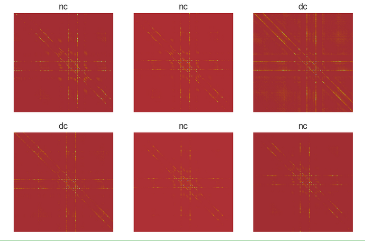
The images are bispectrum images extracted from vibration signals. Each is built from a 4,095 (2¹²-1) data point segment.
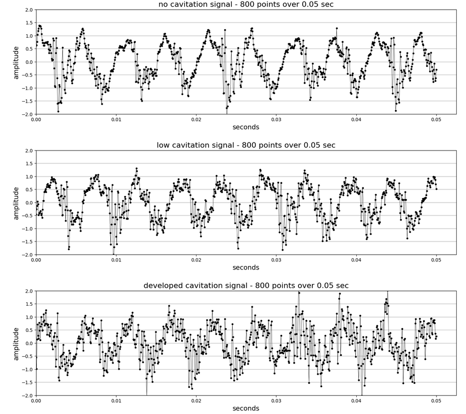
The vibration signals are pump accelerometer data sampled at 16,000 Hz. Three sampling conditions were logged by engineers. Each condition was viewed through the clear pump casing [1].
Three signals:
- No cavitation (nc) — normal pump operation
- Low cavitation (lc) — small cloud of bubbles
- Developed cavitation (dc) — large cloud of bubbles
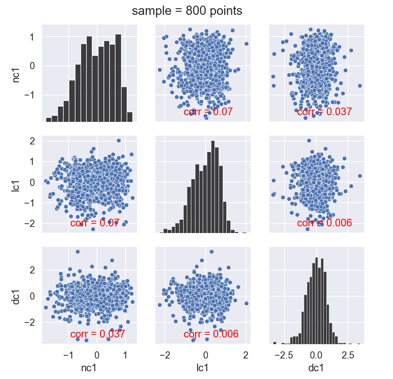
Signal Statistics
Each accelerometer signal has 800,001 data points (that’s 50 seconds at 16,000 Hz). Mean amplitude for each is zero.
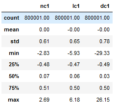
The pairplot of the three conditions shows little correlation between each. The developed cavitation (dc1) condition looks Gaussian in this sample. We revisit the significance of this later.
Get Bispectrum Images
Images and signals are saved in this GitHub repo. To create images yourself, follow this recipe:
- Use joblib.load(‘signals.joblib’) to load the Pandas dataframe with each signal: nc1 and dc1. Chop the signal into non-overlapping 4,095 point segments. With this technique, an 800,000 point signal has 195 images.
- The author’s bispectrum code (Bispectrum2D below) creates the bispectrum image from the signal segment y [2]. Instantiate Bispectrum2D on Line 104. Use freqsample=16,000 and window_name=’hanning’. Hanning is a common window used on unknown signals. To plot the image, use bs2D.plot_bispec_magnitude().
- Save each image. I strongly recommend saving the indices in each file name. This make segregating test images in the future easy. plt.savefig(f’./images/{feature_name}_hanning_{start_idx}-{end_idx}.png’)
- Format images to 224x224 pixels. This is the required size for VGG16.
- Use the VGG16 preprocess_input library:
from tensorflow.keras.applications.vgg16 import preprocess_input
It converts the images from RGB to BGR. Also, “Each color channel is zero-centered with respect to the ImageNet dataset, without scaling.”
Bispectrum2D Python dataclass:
Sidenote on bispectrum2D: The calculation is a standalone implementation— no Python class inheritance touch point nor jargon translation required. The author refactored two Python classes into one dataclass. bispectrum2D automatically produces the range of frequencies from sample frequency.
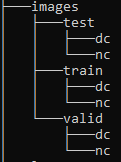
Load Images
Each image class has a folder. The train folder has labeled images to train the model. Valid is for model tuning and metrics during training. Test (a.k.a. holdout) is unseen images to verify model generalization. We’ll do the following binary classification scenario: no cavitation versus direct cavitation [3].
Download the image dataset from the GitHub repo. See the transfer learning Jupyter Notebook coded in Python.
How do we model the images? TensorFlow 2 is the software tool for the image model.
Create the image datasets in Tensorflow. Details below. There are 210 training images and 60 validation images. The images in each are mutually exclusive. Also, the validation images come after the train images in time (the signal is a time series).
Image Datasets for model fitting:
Create Model
Let’s review dataset structure. How will it work with VGG16?
We choose 32 images in a batch. The images are 224 X 224. And the 3 denotes the red, green, and blue color (RGB) channels.
1 train class names: ['dc', 'nc']
2 val class names: ['dc', 'nc']
3 images, xpixels, ypixels, color_channels: (32, 224, 224, 3)
4 labels: (32,)
On Line 3 below, we initialize VGG16. It has nearly 15 million parameters. They are set to non-trainable and therefore are frozen. Also, the final few classification layers are excluded: include_top = False.
Model: "vgg16"
_________________________________________________________________
 Layer (type)                Output Shape              Param #
=================================================================
 input_5 (InputLayer)        [(None, 224, 224, 3)]     0

 block1_conv1 (Conv2D)       (None, 224, 224, 64)      1792

 block1_conv2 (Conv2D)       (None, 224, 224, 64)      36928

 block1_pool (MaxPooling2D)  (None, 112, 112, 64)      0

 block2_conv1 (Conv2D)       (None, 112, 112, 128)     73856

 block2_conv2 (Conv2D)       (None, 112, 112, 128)     147584

 block2_pool (MaxPooling2D)  (None, 56, 56, 128)       0

 block3_conv1 (Conv2D)       (None, 56, 56, 256)       295168

 block3_conv2 (Conv2D)       (None, 56, 56, 256)       590080

 block3_conv3 (Conv2D)       (None, 56, 56, 256)       590080

 block3_pool (MaxPooling2D)  (None, 28, 28, 256)       0

 block4_conv1 (Conv2D)       (None, 28, 28, 512)       1180160

 block4_conv2 (Conv2D)       (None, 28, 28, 512)       2359808

 block4_conv3 (Conv2D)       (None, 28, 28, 512)       2359808

 block4_pool (MaxPooling2D)  (None, 14, 14, 512)       0

 block5_conv1 (Conv2D)       (None, 14, 14, 512)       2359808

 block5_conv2 (Conv2D)       (None, 14, 14, 512)       2359808

 block5_conv3 (Conv2D)       (None, 14, 14, 512)       2359808

 block5_pool (MaxPooling2D)  (None, 7, 7, 512)         0

=================================================================
Total params: 14,714,688
Trainable params: 0
Non-trainable params: 14,714,688
_________________________________________________________________
VGG16 is our base_model. Now insert the final few classification layers (Lines 4–7 and 12–15 below). As always, choosing neural network layer sizes is more art than science. It may require trial-and-error. The good news is the starting point is an awesome base_model.
Model Layers with Classification Layers:
Model: "sequential"
_________________________________________________________________
 Layer (type)                Output Shape              Param #
=================================================================
 vgg16 (Functional)          (None, 7, 7, 512)         14714688

 flatten (Flatten)           (None, 25088)             0

 dense (Dense)               (None, 10)                250890

 dropout (Dropout)           (None, 10)                0

 dense_1 (Dense)             (None, 1)                 11

=================================================================
Total params: 14,965,589
Trainable params: 250,901
Non-trainable params: 14,714,688
_________________________________________________________________
Observe we added 0.25 million Trainable parameters to the model. Before there was zero because all VGG16 parameters are frozen.
Train and Evaluate
We built the model. Now setup the training process. Compile the model (Line 2 below). Metrics are logged with a custom callback (Lines 8–30). The model is fit (Line 33).
The code below loads test_ds — the test dataset.
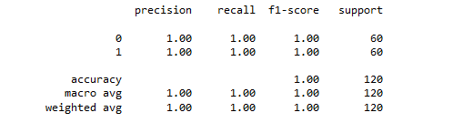
The test image evaluation is 100% accurate (usually — results are stochastic). Only three epochs of training were used. This is the magic of transfer learning.
Loss and Accuracy Metrics
The training loss drops to near-zero after the first epoch per below left plot. Notice training loss is much higher than validation loss after one epoch. Is there data leakage related to the original time-series signal?
Each folder is separate (did not use TensorFlow API to split out validation images). Also, the train, validation, and test data are time-segregated. So train data is before validation data on the timeline. And validation data is before test data.
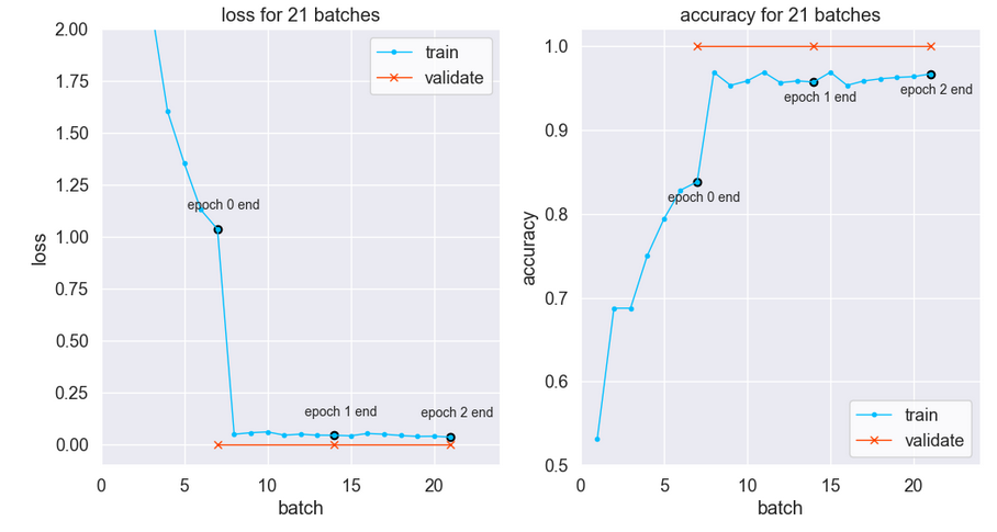
Per the Keras developers, dropout may cause training loss to be higher than “testing” (validation) loss. The full explanation is here. Below the gap between training and validation is narrowed by removing the dropout.
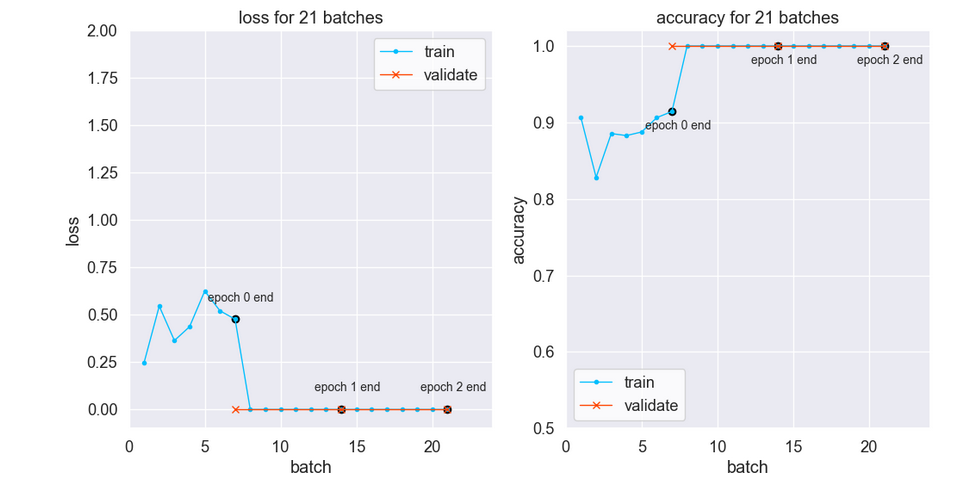
Despite the atypical metrics curves the model generalizes. Indeed, test predictions are 100% accurate — with or without the dropout.
Is a CNN model of this size needed for this task? Probably no! The CNN seems over-parametrized. Indeed, Google Brain research says that a simple two-layer neural network with num_weights = 2 * n_samples + d_dimensions can represent any function [4].
Data Insight
We built an effective binary classification model with nearly 15 million parameters. Job well done? Did we properly explore and understand the signal data?
Time to revisit the 800 point random sample histogram from the Signal Statistics section. Recall the developed cavitation signal looked Gaussian.
Let’s make histograms with more data points. The nc signal below looks bimodal with 8,000 points and 80,000 point samples. In contrast, the dc signal is a unimodal Gaussian curve.
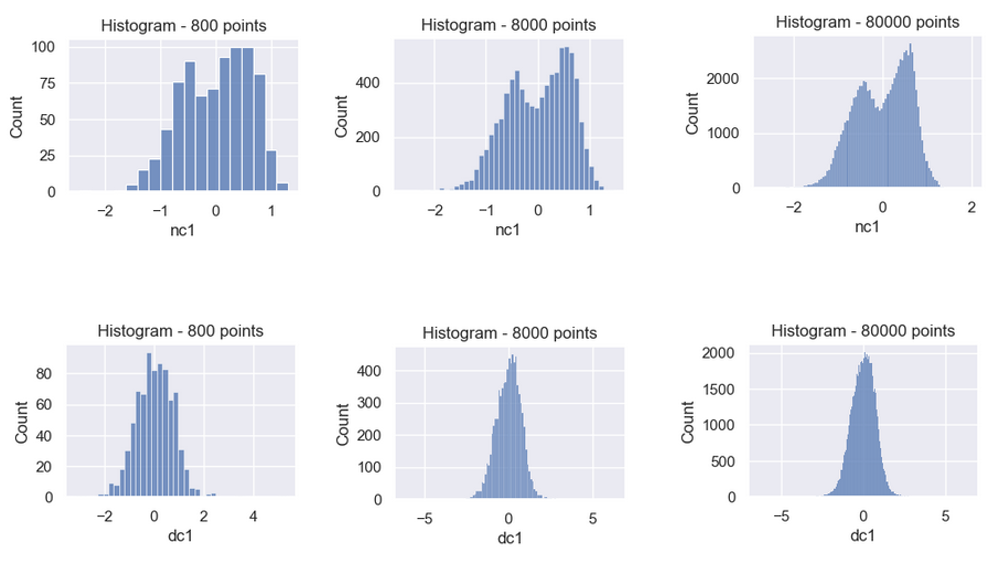
Maybe binary classification is hump counting and no deep learning is needed! Two peaks is no cavitation and one peak is cavitation.
To count peaks, we need to (1) smooth the signal and (2) count local maxima. The volatile signal converts to a smooth curve with Kernel Density Estimation. SciPy has a find_peaks function to count signal local maxima.
from scipy.signal import find_peaks
peaks_num = len(find_peaks(y_kde, height=0.2)[0])
Count peaks by chopping the signal into segments. Again, we expect the no cavitation to have two peaks and developed cavitation to have one peak.
Test 800 point segments peaks first. That is 1,000 independent segments (800*1,000=800,000)per signal. The result is several hundred errors. A poor result.
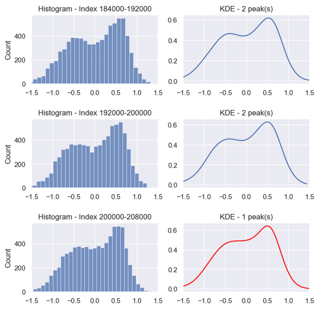
The histogram shows better-defined peaks for 8,000 point segments. It turns out increasing data points boosts accuracy. All segments but one have the correct number of peaks — 99.5% accuracy. That is a big improvement. All that’s required is a bigger sample and curve smoothing [5].
8,000 point segments:
* no cavitation - 100 segments
* developed cavitation - 100 segments
* total segments - 200 segments
accuracy = 99.5% = (200 segments - 1 error) / 200 segments * 100
Conclusion
This project used images from accelerometer signals under two conditions: no cavitation and developed cavitation. We classified the images using a convolutional neural network with nearly 15 million parameters. Of those, 0.25 million were scratch-trained and roughly 14 million are frozen.
The CNN is effective for binary classification. But, there is a simpler option. No images and no large model are required. Just count peaks.
Postscript
For readers looking for more on bispectral analysis, I wrote Fourier and Bispectral Analysis of Signals.
All images unless otherwise noted are by author. Have an awesome day! 😎
REFERENCES
[1] Ali Hajnayeb, "Cavitation Analysis in Centrifugal Pumps Based on Vibration Bispectrum and Transfer Learning", 2021.
Hajnayeb Accelerometer Dataset: nc, lc, dc
[2] Matteo Bachetti, et al., stingray v1.0 code, https://docs.stingray.science, 2022.
[3] Multi-class classification is successful with bispectrum images as per [1]. The neuron count in the final layer increases--one per class. The author chose binary classification to highlight a classification alternative.
[4] Chiyuan Zhang, et al., Understanding Deep Learning Requires Rethinking Generalization, 2017.
[5] Test overlapping time segments to get more confident peak counting works. Increase the number of segments per signal from 100 to 800. Slide the segment window in 1,000 point steps rather 8,000 point steps. The result is two errors total (for both nc and dc). See nc1 indices 199000-207000 and 200000-208000. 1598 correct out of 1600 is 99.875% accuracy, i.e. (1600-2)/1600*100. This is better accuracy fewer segments per signal.
GO TO TABLE OF CONTENTS
Transfer Learning with a One-Dimensional Signal was originally published in Towards Data Science on Medium, where people are continuing the conversation by highlighting and responding to this story.
from Towards Data Science - Medium https://ift.tt/F3R9HTe
via RiYo Analytics


ليست هناك تعليقات