https://ift.tt/7cUwi1L An introduction to the world of causal inference with a hands-on example of using one of its most popular methods to...
An introduction to the world of causal inference with a hands-on example of using one of its most popular methods to answer a causal question

The Causal Question
Understanding the effect of an action on an observed outcome is important for many fields. For example, how does quitting smoking influence weight gain. This type of question seems easy to answer: just look at a people who have quit smoking and compare their average weight change to those who haven’t quit smoking (also known as unadjusted estimation). Let’s say the average weight gain for people that quit smoking is 3 kg and 1 kg for those who haven’t quit. Then we could conclude that quitting smoking causes weight gain. However, this conclusion would be terribly wrong because these groups are not necessarily comparable. There could be confounding factors that are causing this. For example, individuals that quit smoking may feel an increased in appetite and therefore gain more weight.
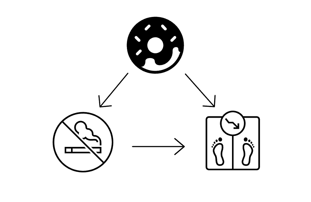
The “gold standard” for estimating causal effects is to conduct randomized control trials. This means that we recruit people and randomly allocate them into exposure groups by, for example, flipping a coin. This wouldn’t work in our example because the last time I checked, telling people to start/quit smoking and then checking how much they weigh in 10 years is both unethical and untimely 😁 (Brady Neal has great examples for this intro to causality).
Let’s look at this mathematically (I promise there are no scary equations ahead!). In the field of causality, the notation Y(a) is the potential outcome for receiving treatment for some individual, meaning what would have happened to them had they received the treatment. So, the average treatment effect of a population (most commonly, the expected difference between two potential outcomes):

As we have seen above, if there is confounding, this is not equal to the associational difference between the two observed groups (quitters vs. persistent smokers):

Getting an unbiased estimate of the treatment effect despite this inequality is the essence of causal inference. This statement becomes true when we identify that the three fundamental assumptions hold (“Causal Inference: What If” by Miguel Hernan chapter 3). Once we concluded the effect is identifiable, we can use a causal effect estimator like IPW to estimate the average outcome given the treatment E[Y|A].
The possible solution
Inverse propensity weighting (IPW) is a method to balance groups by giving each data point a different weight so the weighted distribution of features in each group is similar.
To understand how IPW works its magic we need to know what a propensity score is. Propensity score is just a fancy word for the probability of an individual belonging to a treatment group A given its characteristics X:

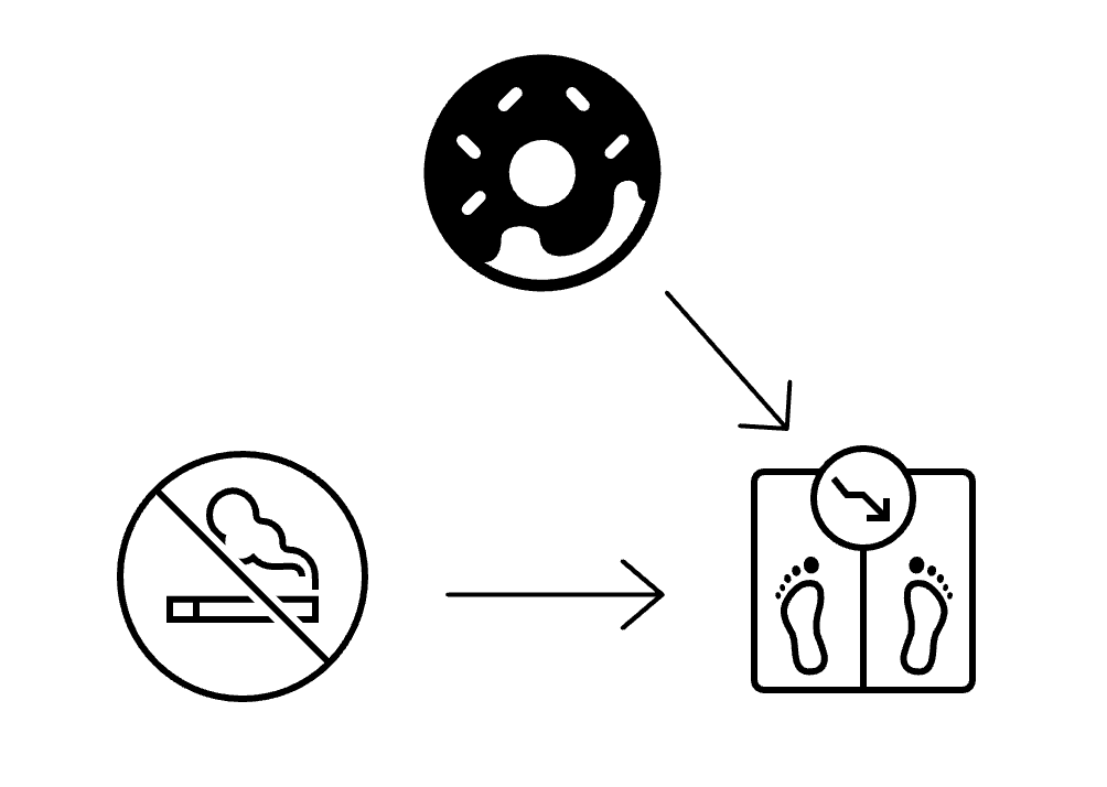
This probability can be estimated with any ML model of your heart desires💕 (Although we can technically use any ML model, it’s important to avoid overfitting by using very complex models. To understand this further check out this notebook). Once we estimate this probability, the weight that is given to each sample is simply the inverse of the propensity score! (For a more detailed explanation of IPW have a look at chapter 12 of “Causal Inference: What If” by Miguel Hernan) The re-weighting creates a pseudo population that no longer has the underling confounding association, this is equal to removing the arrow in the causal graph:
When to choose IPW
All causal models need to have multiple assumptions for them to be reliable:
- There is confounding — both treatment assignment and outcome are influenced by some covariates. If not, then no corrections for confounding are required.
- There are no unmeasured confounders — all the confounding variables are accounted for in your model.
- There are no positivity violations — each sample has a positive probability of belonging to both treatment groups.
Choosing IPW over other causal models should be when:
- You do not need individual level predictions, only the average across the entire population.
- Since IPW models the treatment assignment given the covariates, you need to feel you understand the treatment assignment procedure well.
So, this is all great, but how is it done in practice? This is where causallib comes in play.
Finding the causal effect with causallib
Causallib is an open-source python package that allows you to plug in any sklearn ML model and get causal predictions as long as the assumptions on the data are valid. The package can execute multiple causal models like IPW, outcome models, and Double Robust methods, and provide a suite of evaluations for assessing models’ performance. It is available on PyPi and can be installed by running pip install causallib. The code shown here was run using version 0.9.0.
We will look at the effect of quitting to smoke on weight change for this example. The data is from 1566 cigarette smokers aged 25–74 who had a baseline visit and a follow up 10 years later. The treated individuals (A=1) are those that reported quitting smoking before the follow up visit and the untreated (A=0) otherwise. The data is taken from “Causal Inference: What If” by Miguel Hernan and can be found here.
Our goal is to estimate the average causal effect of smoking cessation (the treatment) A on weight gain (the outcome) Y. From looking at the data, the average weight gain was 4.5 Kg in the quitters and 2.0 Kg in the non-quitters. The difference is therefore 2.5 Kg with a 95% confidence interval from 1.7 to 3.4. This type of estimation is called “unadjusted estimation” as I referenced in the beginning of this post. So, you might think, great we found the answer to our question! But this does not tell us what the effect of smoking cessation is on weight loss, it is simply reporting the difference in weight changes between the groups of quitters and non-quitters. If quitting smoking was assigned randomly, we could take this as a valid estimate of the effect. But since the likelihood of quitting is itself affected by the individual’s covariates, simply comparing averages of the two groups produces a biased estimation of the treatment effect. In order to debias the estimation, we need to bias adjust for confounding. So, let’s try again with the help of IPW.
The IPW from causallib is a “meta learner.” It wraps a generic binary outcome prediction model and uses it to estimate the propensity and estimate the effect. The underlying learner can be anything as long as it supports the sklearn interface. For this example, we will use good old Logistic regression as our core estimator because of its relative robustness to overfitting and had comparable performance to other models when I experimented on this data.
First, we instantiate the IPW class with our chosen learner and fit it to the data:
- data.X is the feature matrix for all subjects
- data.a is the treatment of each subject (did/didn’t quit smoking)
Next, we estimate the average balanced outcome for each treatment group. We will be using the Horvitz–Thompson estimator which is the inverse propensity weighted average of Y.
This function outputs a series (‘outcomes’) with the average potential outcome predicted for both treatment groups.
Lastly, an “effect” is a contrast of two potential outcome, and we have to freedom to specify treatment effect in both the additive (diff) and the multiplicative (ratio) scale. We will use the difference:
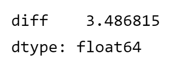
We can see that on average, individuals who quit smoking gained 3.4 Kg, which is different than the result we got with unadjusted estimation (2.5 kg). This is the same result as can be seen in “Causal Inference: What If” by Miguel Hernan page 152.
Evaluation with causallib
The key difference between causal inference models and ML models is that in supervised learning we almost always have ground truth. Let’s say we are training a classifier to predict the number of Kg lost ten years after quitting smoking. When we test the model, we can see which samples had large residuals because they are labelled. This ability to check how well your model really works doesn’t exist here because of the “fundamental problem of causal inference” (explained deeply in Brady Neal Introduction to Causal Inference 2.2). In a nutshell, we can never directly verify if the potential outcomes are correct because we cannot observe two different outcomes, under two different actions, in the same person. A person can’t both quit and not-quit smoking.

Even though you cannot evaluate the ground truth in causal inference, causallib provides several evaluations that help you to detect problems with your model.
The evaluate function enables us to cross-validate models, create evaluation plots and calculate scores. First, we specify the evaluation metrics we are interested in for our model. The evaluation is done using cross-validation and refitting the model on each fold.
We will generate a new model that hasn’t been fit to the data before and check how well it preforms.
The Love Plot
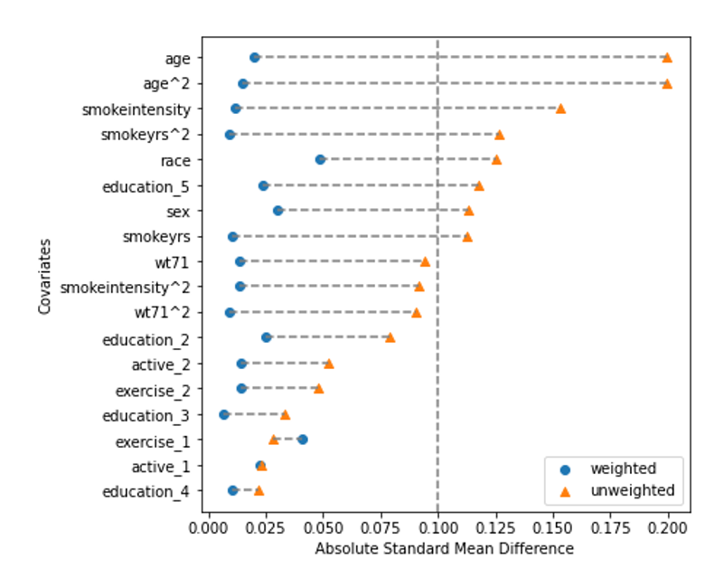
The Love plot calculates the standardized mean difference between groups for each covariate before and after weighting. We hope that after weighting the difference for all covariates will be smaller than some threshold, usually 0.1. This result indicates that the weighting successfully created a pseudo population where the covariates are equally distributed between the two groups.
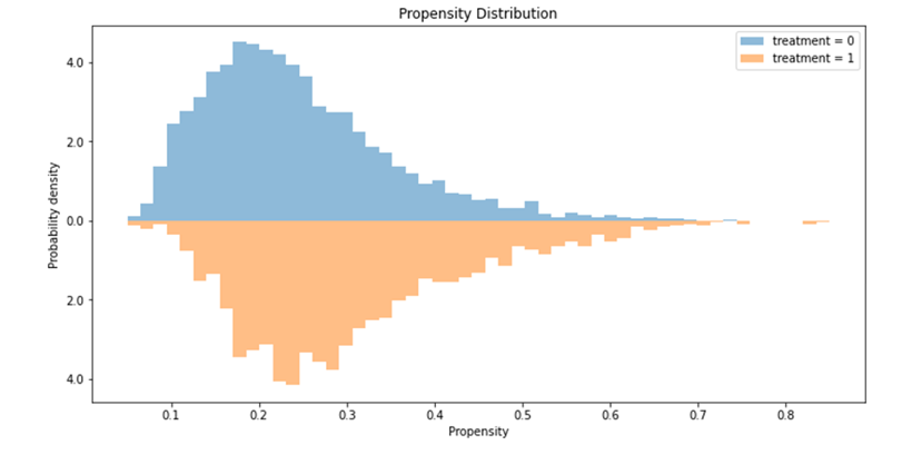
Propensity Distribution Plot
Another important evaluation plot is the distribution of the propensity scores for both treatment groups. Ideally the two distributions should be overlapping but not identical. If they are identical, that would mean the two treatment groups are indistinguishable given the covariates. This also confirms that there isn’t a positivity violation as every subject has a non-zero probability of being in either treatment group and the distributions overlap (have a look at this notebook for an example of a positivity violation).
Discussion
In this post we showed how to use causallib’s IPW to get some insight about the causality between a treatment and its outcome. The causallib package enables us to leverage the rich library of Scikit-Learn models and evaluation metrics in order to make causal estimations, making it easy to incorporate these types of questions as part of any data exploration process.
There are many more causal models that can be used like standardization, double robust models, X-learners and more. Each have different hyperparameters to tune for personalizing the estimation as you like.
some helpful links :
- Causallib example IPW notebook
- Causallib GitHub
- “Causal Inference: What If” by Miguel Hernan
- Causal Inference course by Brady Neal
- “Causal Inference for the Brave and True” by Matheus Facure Alves
Thanks to Michael M Danziger and Ehud Karavani for helping create this post!
Hands-On Inverse Propensity Weighting in Python with causallib was originally published in Towards Data Science on Medium, where people are continuing the conversation by highlighting and responding to this story.
from Towards Data Science - Medium https://ift.tt/luakTSm
via RiYo Analytics

ليست هناك تعليقات