https://ift.tt/h3u8Als Can you use the pipe operator for pandas dataframes? plydata: Is the spring of pandas approaching? Photo by Biegun...
Can you use the pipe operator for pandas dataframes?

Introduction
Piping can be a powerful tool in exploring data frames. R’s %>% pipe operator shows this very well. But what about Python and pandas dataframes? Why does it not offer anything like that?
Most of those who move from R to Python (like me) feel that Python lacks a pipe operator, or at least one as powerful as R’s %>%. In R, it’s included in tidyverse (Wickham, 2019), the collection of extremely powerful tools for manipulating data — although the truth is that it was introduced in the magrittr R package.
The truth is that Python does come with something similar, though not (yet) as powerful. In fact, there are several modules that offer a pipe operator to work with. An interesting one is the Pipe package, which aims to offer similar piping as in functional programming languages, such as F# or Haskell. However, it’s not designed to work with data frames; thus, as it is interesting and useful in some other contexts, we will talk about it some other time. Today, however, we’re talking about data frames. The %>% operator in R — so powerful and so much loved — was designed to work with data frames (and similar types, like tibble, Müller and Wickham 2021), so it does not work like pipe operators in functional languages.
In fact, there have been several approaches to achieve this, and quite an interesting one among them is plydata. Today, we will discuss its basics and its pipe operator, >>. After this basic introduction, you should be ready to decide whether you like this solution or not.
The first steps into plydata
Of course, our first step should be the installation of a virtual environment with the required modules. I will be using pydataset==0.2.0 (even if old, the package still offers datasets, so it should be working fine) and plydata==0.4.3. plydata is also getting a little old, since the last version is from 2020, but I see that its repository is still active, so I think we should expect an update sometime soon.
Once we’ve created the virtual environment with these packages, we can use its Python installation. Here’s what we’ll need:
I will use the iris data set, which is extremely popular in various disciplines, including classification and data visualization. I have used it myself in quite a few scientific articles I wrote about statistics and data visualization; I even co-authored an article (Kozak and Łotocka 2013) about this very data set.
plydata offers quite a few useful functions, but in this introductory article, we will discuss just a couple of them. First, let’s import the dataset from the pydataset package:
In the data, 150 observations are grouped into three Iris species (I. versicolor, I. virginica, and I. setosa), each of them having four variables. Now, our first use of plydata: Let’s print the first five rows per each species:
or, which to me is much more readable,
It’s just the beginning. I will explain the group_by() function later, though I think its name says what it does. pandas users will immediately know what it is about; and in fact, pandas users will more often than not rather quickly understand what plydata functions do.
Above, the head() function takes the first n rows of data. Let’s go on, but we must first rename the columns. We certainly don’t need plydata for that:
Of course, we could do it in a number of ways, like with the pandas.DataFrame.rename() method. OK, we’re almost ready to go, but since we will calculate coefficients of variation, we first need to define a function for doing so:
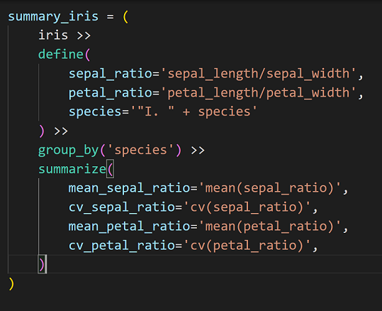
Now, onto business. The short code below shows the power and readability of plydata:
Before reading further, please take a moment to read the code above and understand what it does; for the moment, please ignore the line I commented out, and we will return to it later.
The key lies in the pipe operator, >>, which serves the same purpose as R’s pipe operator from magrittr, that is, %>%. Yes, I wrote from magrittr, because this very package introduced the %>% operator, so heavily used by the tidyverse environment.
In general, pipes help you run functions on your dataset in sequence. You know the idea, since Pythonistas can use the dot in similar chains, like in my_string.lower.replace('gz', 'z'), or in pandas. I don’t think I have to convince you that such a functionality can come quite handy, though it has one quite significant limitation, which I will discuss later.
When you’re done pondering the code, let’s go through it line by line:
* iris means we’re starting off with the iris data frame (yes, plydata works with pandas.DataFrames, and so it will not work with generators, for instance).
* The define() function, of course, defines new variables; here, sepal_ratio and petal_ratio. Here, it also redefines species by adding “I. ” at the beginning: This is how biologists write species names.
* The commented line: We do not need to select any variable here, actually, but I wanted to show you that we could if we wanted to get rid of some of them (as we often do). Uncommenting this line would change nothing, since there are no additional variables in the iris data set. Here, we would drop columns with either width or length in their names.
* Now we group the data by species. These eight characters combined into group_by() offer so much power that it is difficult to imagine. What it does is: Everything that will be done after that line will be done per group. So, if we calculate the mean of a variable, we will get the means for each species (as species make groups).
* summarize() aims to, unsurprisingly, summarize the data. Here, we determine the mean (from the statistics module) and the coefficient of variation (using the function we defined above).
Look at the results:
I did not need the query() function, but since it’s so important, let me show you how it works. Say we want to find those samples in which sepals were relatively wide; here, we’ll query for at least 75% of its length:
We can add other conditions, using the and (you can also use or, of course) operator (since many rows meet this condition, let’s take only the first three):
It’s difficult for me to assess how readable such plydata code is for you, because I’ve been using R’s piping for a long time. Hence I read it just like a written text, though I do remember that at first I needed to get used to this syntax. These days, it’s really clear to me, at least at this level — because it can be much more difficult to understand (and debug!) when combined with complex functions.
Limitations
I have just mentioned the biggest limitation of piping: debugging. Indeed, debugging can be difficult. Sometimes it’s best to unpipe the code; you can also add some prints, but interactive debugging with pipes requires more work.
In addition, sometimes you can do more with pandas, especially when your knowledge of plydata is still poor. Frankly, I often ended up with code mixing up plydata and pandas syntax. Maybe such code was not as nice as pure plydata code, but it still was fine and clearer than pure pandas .
Conclusion
A couple years ago, R changed the data exploration world by including the pipe operator, %>%. It is so powerful and offers so many possibilities that it is difficult to imagine nowadays R without dplyr and piping R commands. In my eyes, it was even the biggest game changer in R’s history.
Why does Python’s pandas make us live without a pipe operator? When I moved from R to Python, it was a huge surprise to me, and not a good one. Nonetheless, since others have worked to solve this issue, here we are, with plydata and its >> operator to help us operate pandas data frames.
I think much of the power of chaining commands via a pipe comes from using one assignment instead of many. Since in this article I have shown the basics of plydata, I did not include long chains. The truth is, however, that even long chains can be easy to read, and instead of using, say, ten assignments, you need just one. Besides, the vertical organization of commands (except for very short ones, which can be organized in one line) helps our eyes to follow what is being done, step by step, in a well organized and easily readable form. Note (for instance, in the image above) that the organization of such code also matches with Python’s indentation rules.
I have to admit that R’s syntax for chaining commands with the %>% operator seems a little easier and nicer to me than that with the >> operator of plydata. This, however, can result from all the years I have spent programming in R. But operating on dataframes is so much easier with pipes that it’s really worth learning this functionality, even if it looks a little complicated at first glance. But the time spent on plydata will pay off some day, sooner or later.
While plydata is still behind thetidyverse environment in development, if data scientists working with pandas start using it a lot, I believe its development will rapidly accelerate; and then, who knows, maybe in some time, piping will become the main tool for handling data frames in Python, just as it is in R. This would be beneficial for all of us data scientists, for the simple reason that piping enables one to do incredible data manipulations with so readable syntax.
I showed you just some basics of using plydata and dataframe piping, and I hope I have convinced you it helps a lot during the exploration of data frames. In next articles, we will go deeper into the package, as the pipe operator constitutes the essence, but plydata certainly offers a lot more than that. It offers various functions that enable the user to manipulate dataframes in a variety of ways.
References
Bache, S.T., & Wickham, H. (2020). magrittr: A Forward-Pipe Operator for R. R package version 2.0.1. https://CRAN.R-project.org/package=magrittr
Kozak, M., & Łotocka, B. (2013). What should we know about the famous Iris data. Current Science, 104(5), 579–580. [Available here](https://ift.tt/1zmwTYg)
Müller, K., & Wickham, H. (2021). tibble: Simple Data Frames. R package version 3.1.2. https://CRAN.R-project.org/package=tibble
Wickham et al. (2019). Welcome to the tidyverse. Journal of Open Source Software, 4(43), 1686, https://doi.org/10.21105/joss.01686
plydata: Piping for pandas was originally published in Towards Data Science on Medium, where people are continuing the conversation by highlighting and responding to this story.
from Towards Data Science - Medium https://ift.tt/7knfGSp
via RiYo Analytics


No comments