https://ift.tt/KStnP8W Hands-on guide to implement and validate self-training using Python Photo by Sander Weeteling on Unsplash Semi...
Hands-on guide to implement and validate self-training using Python

Semi-Supervised Learning is an actively researched field in the machine learning community. It is typically used in improving the generalizability of a supervised learning problem (i.e. training a model based on provided input and ground-truth or actual output value per observation) by leveraging high volumes of unlabeled data (i.e. observations for which inputs or features are available but a ground truth or actual output value is not known). This is usually an effective strategy in situations where availability of labeled data is limited.
Semi-Supervised Learning can be performed through a variety of techniques. One of those techniques is self-training. You can refer to Part-1 for details on how it works. In a nutshell, it acts as a wrapper which can be integrated on top of any predictive algorithm (that has the capability to generate an output score via a predict function). The unlabeled observations are predicted by the original supervised model and the most confident predictions by the model are fed back for re-training the supervised model. This iterative process is expected to improve the supervised model.
To get started, we will set up a couple of experiments to create and compare baseline models which will use self-training on top of regular ML algorithms.
Experiment setup
While semi-supervised learning is possible for all forms of data, text and unstructured data are the most time-consuming and expensive to label. A few examples include classifying emails for intent, predicting abuse or malpractice in email conversations, classifying long documents without availability of many labels. The higher the number of unique labels expected, the harder it gets to work with limited labeled data. Hence, we take the following 2 datasets (in increasing order of complexity from a classification perspective):
IMDB reviews data: Hosted by Stanford, this is a sentiment (binary- positive and negative) classification dataset of movie reviews. Please refer here for more details.
20Newsgroup dataset: This is a multi-class classification dataset where every observation is a news article and it is labeled with one news topic (politics, sports, religion and so on). This data is available through the open source library scikit-learn too. Further details on this dataset can be read here.
Multiple experiments are conducted using these 2 datasets at different volumes of labeled observations to get a generalized performance estimate. Towards the end of the post, a comparison is provided to analyze and answer the following questions:
- Does self-training work effectively and consistently on both algorithms?
- Is self-training suitable for both binary and multi-class classification problems?
- Does self-training continue to add value as we add more labeled data?
- Does adding higher volumes of unlabeled data continue to improve model performance?
Both datasets can be downloaded from their respective sources provided above or from Google Drive. All the codes can be referenced from GitHub. Everything has been implemented using Python 3.7 on Google Colab and Google Colab Pro.
To evaluate how each algorithm would do on the two datasets, we take multiple samples of labeled data (low volume to high volume of labeled data) and apply self-training accordingly.
Understanding the input
Newsgroup training dataset provides 11,314 observations spread across 20 categories. We create a labeled test dataset of 25% (~2800 observations) from this and randomly split the remaining into labeled (~4,200 observations are considered with their newsgroup label) and unlabeled observations (~4,300 observations are considered without their news group label). Within each experiment, a portion of this labeled data is considered (starting from 20% and going upto 100% of labeled training volume) to see whether increase in the volume of labeled observations in training leads to performance saturation (for self-training) or not.
For the IMDB dataset, two training batches are considered: (1) using 2,000 unlabeled observations and (2) 5,000 unlabeled observations. Labeled observations used are 20, 100, 400, 1000, 2000. Again, the hypothesis remains that increase in number of labeled observations, would reduce the performance gap between a supervised learner and a semi-supervised learner.
Implementing the concepts of self-training and pseudo labelling
Each supervised algorithm is run on the IMDB movie review sentiment dataset, and the 20NEWSGROUP datasets. For both datasets, we are modeling for a classification problem (binary classification in the former case and multi-class in the latter case). Every algorithm is tested for performance at 5 different levels of labeled data ranging from very low (20 or so labeled samples per class) to high (1000+ labeled samples per class).
In this article, we will perform self-training on a couple of algorithms — logistic regression ( through sklearn’s implementation of sgd classifer using a log loss objective) and vanilla neural network (through sklearn’s implementation of mulit-layer perceptron module).
We’ve already discussed that self-training is a wrapper method. This is made available directly from sklearn for sklearn’s model.fit() methods and comes as part of the sklearn.semi_supervised module. For non-sklearn methods, we first create the wrapper and then pass it over to pytorch or Tensorflow models. More on that in later.
Let’s start by reading the datasets:
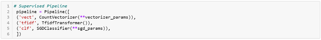
Let’s also create a simple pipeline to call the supervised sgd classifier and the SelfTrainingClassifier using sgd as the base algorithm.
Tf-Idf — logit classification
The above code is pretty straightforward to understand, but lets quickly break it down:
- First, we import the required libraries and use a few hyperparameters to set up logistic regression (regularization alpha, regularization type being ridge, and a loss function which is log loss in this case).
- Next, we provide count-vectorizer parameters where n_grams are made of minimum 1 word and maximum 2 tokens. Ngrams, that appear in less than 5 documents OR in over 80% of corpus, are not considered. A tf-idf transformer takes the count vectorizer output and creates a tf-idf matrix of the text per document-word as features for the model. You can read more about count vectorizer and tf-idf vectorizer here and here respectively.
- Then, we define an empty DataFrame (df_sgd_ng in this case) that stores all performance metrics and information on labeled and unlabeled volumes used.
- Next, in n_list, we define 5 levels to define what percent of training data is passed as labeled (from 10% in increment of 10% up to 50%). Similarly, we define two parameter lists to iterate on (kbest and threshold). Usually, training algorithms provide probability estimates per observation. Observations where the estimate is above a threshold, are considered by SelfTraining in that iteration to be passed to the training method as pseudo labels. If a threshold is unavailable, kbest can be used to suggest that top N observations based on their values should be considered for passing as pseudo labels.
- The usual train-test split is followed next. Post this, using a masking vector, training data is built by first keeping 50% of data as unlabeled and within the remaining 50% data, using n_list, labeled volume is considered in increments (i.e. 1/5th of total labeled data is added incrementally in each subsequent run till all of labeled data is used). The same labeled training data is each time used independently for regular supervised learning as well.
To train the classifier, a simple pipeline is built: Starting with (1) count vectorizer to create tokens followed by (2) TfIdf transformer to convert tokens into meaningful features using the term_freq*Inverse_doc_freq calculation. This is then followed by (3) fitting a Classifier to the TfIdf matrix of values.
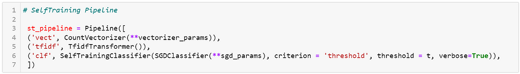
Everything else remaining the same, the pipeline for self-training is created and called where instead of fitting a classifier directly, it is wrapped into SelfTrainingClassifier() as follows:
Finally, for each type of classifier, the results are evaluated on test dataset via a function call to eval_and_print_metrics_df()

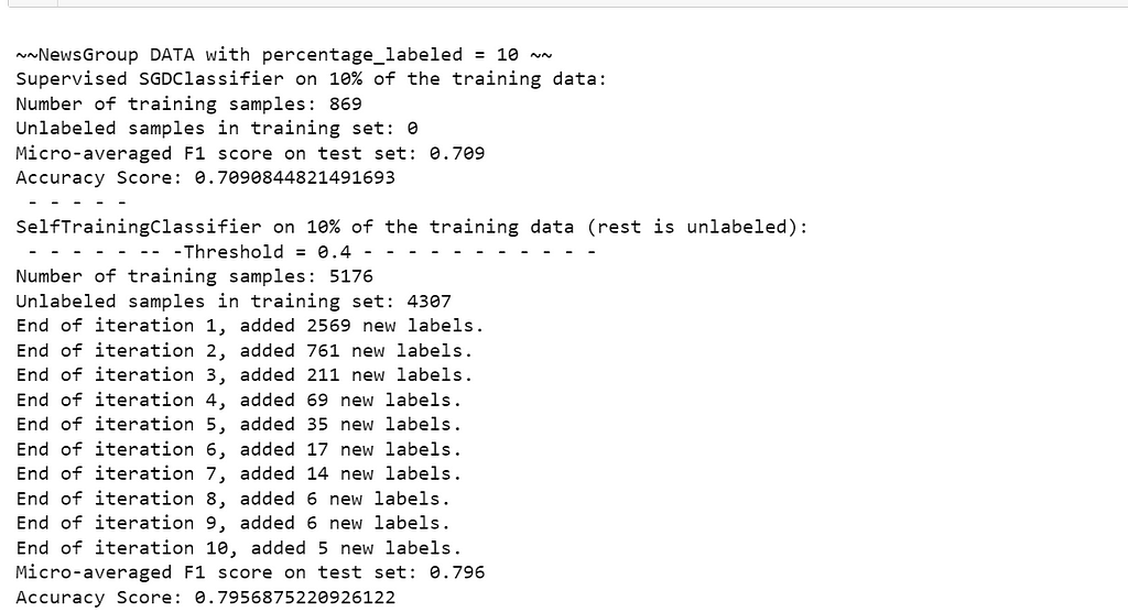
The following image shows how the console output looks like when running supervised classification followed by self-trained classification:
Tf-Idf — MLP classification
The self-training for MLP classifier (i.e. a vanilla feed forward neural network) is done in exactly the same manner with the only differences coming up in the classifier’s hyperparameters and its call.
Note: MLP from scikit-learn implementation is a non-GPU implementation and thus large datasets with very dense layers or deep networks will be very slow to train. The above is a simpler setup (2 hidden layers with 100 and 50 neurons and max_iter=25) to test the generalizability of self-training. In Part-3, we will be implementing all of self training based on ANNs, CNNs, RNNs and transformers using GPU support on Google Colab Pro leveraging Tensorflow and Pytorch.
For MLP, the first console output has been provided below:
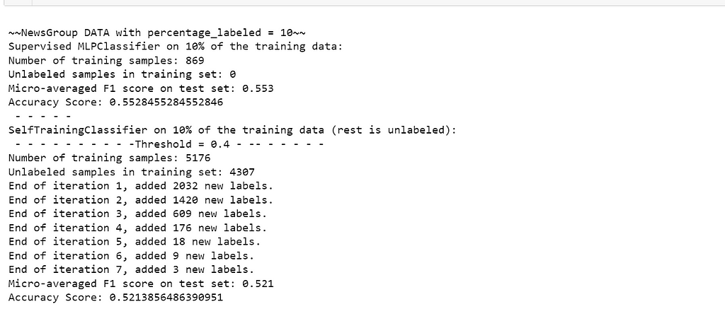
The above console output implies that upon running a supervised classifier first, the model was fitted on 10% of training data (as labeled). The performance on test data for such a classifier is 0.65 of Micro-F1 and 0.649 of accuracy. Upon starting self training with 4,307 unlabeled samples in addition to existing labeled volumes, pseudo labels of unlabeled observations will be pushed for next iteration of training only if their output probability for any one class is at least as high as the threshold (0.4 in this case). In first iteration, 3,708 pseudo labels are added to 869 labeled observations for a 2nd training of the classifier. On subsequent predictions, another 497 pseudo labels are added and so on till no more pseudo labels can be added.
To make comparison metrics consistent, we create a simple utility here. This takes the training and test dataset along with the fitted classifier (which changes based on whether we are using supervised learning or semi-supervised learning in that evaluation step) and in case of semi-supervised learning, whether we are using threshold or kbest (when direct probability outputs are not possible like with Naive Bayes or SVM). This function creates a dictionary of performance (micro-averaged F1 and accuracy) at different levels of labeled and unlabeled volume alongside information on threshold or kbest, if used. This dictionary is appended into the overall performance DataFrame (like df_mlp_ng and df_sgd_ng shown in earlier Github gists).
Finally, lets see the full length comparison outputs and realize what we’ve found so far when different volumes of labeled observations are considered with self-training at different thresholds.
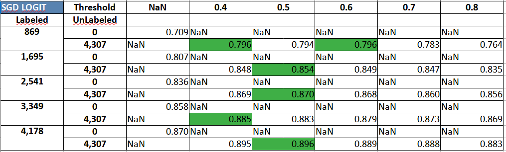
The table above for logistic regression can be explained as follows:
We start with 5 sizes of labeled dataset (869, 1695 and so on till 4178). Using each iteration of labeled data, we train a supervised classifier model first and document the model performance on test data (Accuracy numbers with Threshold column = NaN). Within the same iteration, we follow up with adding 4,307 samples of unlabeled data. The pseudo labels generated are selectively passed into the supervised classifier but only if they exceed the pre-decided probability threshold. In our experiments, we worked with 5 equally spaced thresholds (0.4 to 0.8, with step size of 0.1). The accuracies for respective threshold based self-training is reflected per labeled volume iteration. In most cases, it can be seen that using unlabeled data leads to a performance improvement (but, in general, as labeled volume increases, the boost from self-training, and in general from other semi-supervised methods also, saturates).
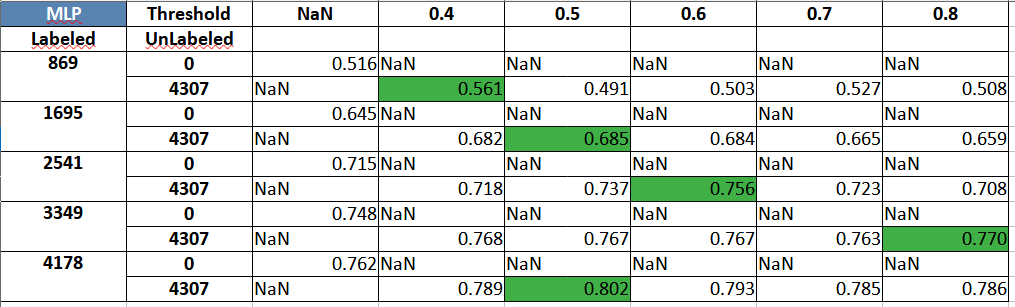
The following table provides a comparison using a MLP:
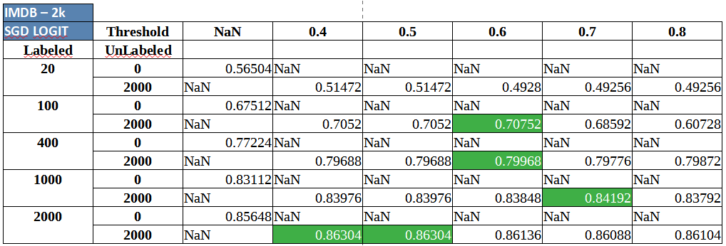
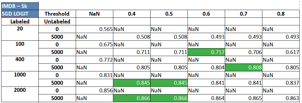
Similar tables are produced below for the IMDB sentiment classification dataset. The code continue to be in the same notebook and can be accessed here.
IMDB review sentiment classification using Semi-Supervised Logistic Regression:
IMDB review sentiment classification using Semi-Supervised MLP/ Neural Network:
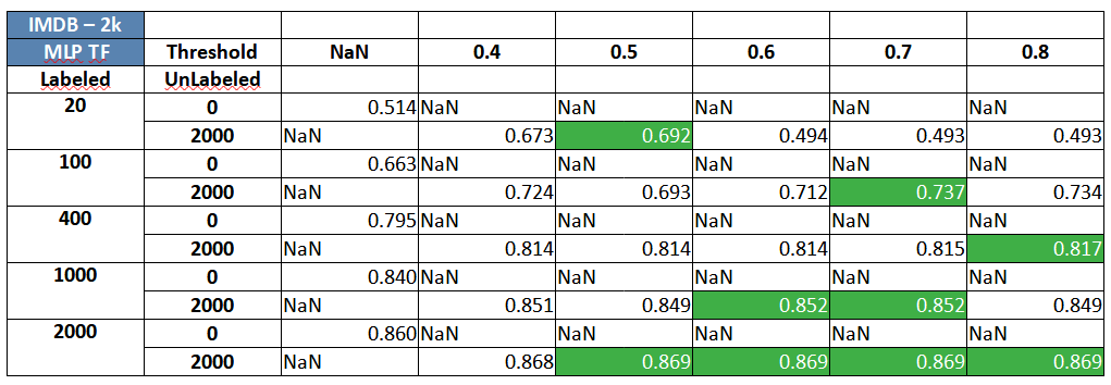
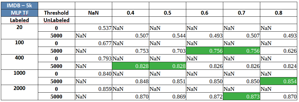
Two key and consistent insights that can should be clearly observed are:
- Self-training, almost always, seems to provide a small and varied, but definite boost at different volumes of labeled data.
- Adding more unlabeled data (2,000 vs. 5,000 unlabeled observations) seems to provide delta improvement in performance consistently.
Many of the results, across datasets and algorithms above, highlight something slightly odd as well. While there is a performance boost in most situations where self training is involved, the results that sometimes adding labels at mid-low confidence pseudo labels (probability around 0.4 to 0.6) along with high confidence labels leads to a better classifier overall. For mid-high thresholds, it makes sense because using very high thresholds would basically imply working with something close to supervised learning but success with low thresholds goes against normal heuristics and our intuition. In this case, it can be attributed to three reasons- (1) The probabilities are not well calibrated and (2) the dataset has simpler cues in the unlabeled data which are getting picked up in the initial set of pseudo labels even at lower confidence levels (3) the base estimator itself is not strong enough and needs to be tuned to a strong extent. Self-training should be applied on top of a slightly tuned classifier.
So, there you have it! Your very first set of self training pipelines that can leverage unlabeled data and a starter code to generate a simple comparative study on how much volume of labeled data and what threshold for pseudo labels could improve model performance significantly. There is still a lot left in this exercise - (1) calibrating probabilities before passing them to self-training, (2) playing with different folds of labeled and unlabeled datasets to have a more robust comparison. This should hopefully serve as a good starting point when working on self-training.
All the codes used in this post can be accessed from GitHub.
Sneak peak into SOTA using GANs and Back-Translation
In recent years, researchers have started leveraging data augmentation to improve semi-supervised learning through use of GANs, and BackTranslation. We would like to understand these better and compare such algorithms against self-training employed on neural networks and transformers through the use of CNNs, RNNs, and BERT. The recent SOTA techniques for semi-supervised learning have been MixText and Unsupervised Data Augmentation for Consistency Training which would also be topics touched upon in Part-3.
Thanks for reading and see you in the next one!
The 3-part series, including this article, has been a joint work between Abhinivesh Sreepada, who is a passionate NLP data scientist with a master’s graduate from Indian Institute of Sciences (IISC), Bengaluru-IN and Naveen Rathani, who is an experienced machine learning specialist and a data science enthusiast.
References:
[1] https://scikit-learn.org/stable/modules/generated/sklearn.linear_model.SGDClassifier.html
[4] https://ai.stanford.edu/~amaas/data/sentiment/
[5] http://kdd.ics.uci.edu/databases/20newsgroups/20newsgroups.html
Improve Model Performance Using Semi-Supervised Wrapper Methods was originally published in Towards Data Science on Medium, where people are continuing the conversation by highlighting and responding to this story.
from Towards Data Science - Medium https://ift.tt/1q0eCcu
via RiYo Analytics


ليست هناك تعليقات