https://ift.tt/MrklxZu Translating observations into interventions This is the 3rd article in a series on causal effects . In the last pos...
Translating observations into interventions
This is the 3rd article in a series on causal effects. In the last post, we reviewed a set of practical approaches for estimating effects via Propensity Scores. The downside of these approaches, however, is they do not account for unmeasured confounders. By the end of this article we will see how we can overcome this shortcoming. But first, we need to take a step back and reevaluate how we think about causal effects.
Key Points:
- The do-operator is a mathematical representation of an intervention
- An intervention is the intentional manipulation of a data generating process
- Using Pearl’s Structural Causal Framework we can estimate the effect of interventions using observational data
Up to this point in the series, we have (for the most part) taken a classic statistical approach to the computation of causal effects. In other words, we split our data into two populations (e.g. treatment and control group) and compared their means. However, there is a more robust way to think about things.
Master of Causality Judea Pearl frames things in what he calls a Structural approach to causality [1]. A central piece of this approach is the so-called do-operator.
We first saw the do-operator in the article on causal inference. There, the operator was introduced as a mathematical representation of an intervention which enables us to compute causal effects. Here we will explore this notion in greater detail.
Average Treatment Effect with the Do-Operator
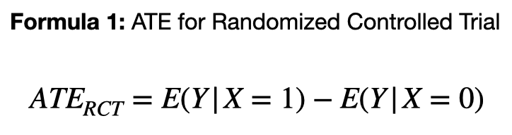
In the first post of this series, we defined the Average Treatment Effect (ATE) for a randomized controlled trial, as the difference in expected outcomes between two levels of treatment. In other words, we compare the expectation value of the outcome variable (e.g. has headache or not) conditioned on treatment status (e.g. took pill or not). This is one of the most widely used approaches to quantifying causal effects.
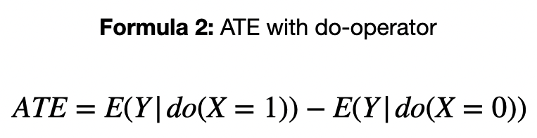
Alternatively, ATE in Pearl’s formulation is defined as the difference in expected outcomes between two levels of intervention [1]. This is where the do-operator comes in.
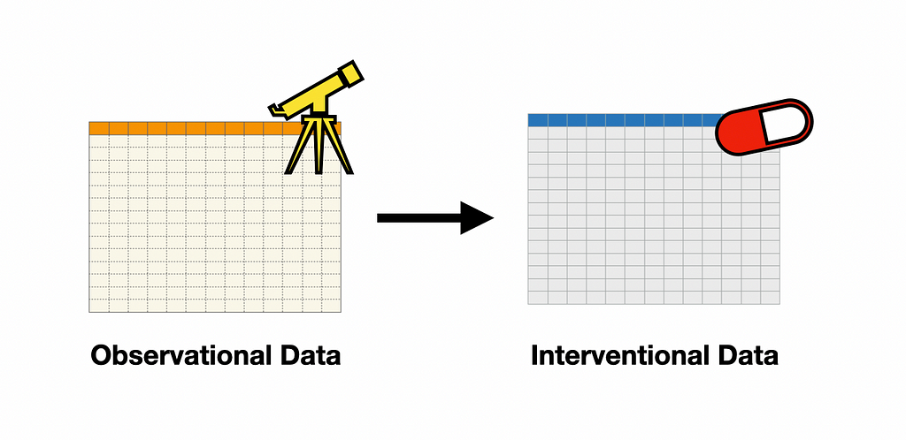
Observational vs Interventional Distributions
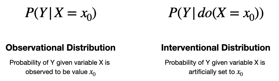
The key difference between P(Y | X=x)) and P(Y | do(X=x)), is that the first specifics the probability of Y given a passive observation of X=x, while the latter represents the probability of Y given an intervention in X.
Here, I will call a distribution containing the do-operator an interventional distribution (e.g. P(Y | do(X=1))), while one without it, I will call an observational distribution. Note: this is similar to the distinction made in the last blog between observational and interventional studies.
Formula 1 vs Formula 2
In the context of a Randomized Controlled Trial (RCT), Formula 1 and Formula 2 are equivalent. Since treatment assignments are intentionally (and carefully) manipulated by experimenters. However, once we move outside of an RCT (or something similar), Formula 1 is no longer valid, but Formula 2 is.
In this way, we can think of Formula 2 as a generalization of Formula 1. This new formulation provides us a clearer picture of causal effects. It helps move us away from ad hoc equations for specific contexts, to a more general (and powerful) framework. In the next section, we will see the power of this formulation in practice.
Identifiability
Connecting observational and interventional distributions in 3 steps
While theory and abstractions can be helpful, at some point we need to connect them to reality (i.e. our data). In the context of causality, this raises the question of identifiability. In other words, can the interventional distribution be obtained from the given data? [1]
As I alluded to earlier, if we have data from an interventional study (e.g. an RCT), we indeed have the interventional distribution (that’s what we painstakingly measured). But what if we only have observational data?
Lucky for us, this problem has already been solved by Pearl and colleagues [1]. The solution can be broken down into 3 steps.
Step 1 — Write down a causal model
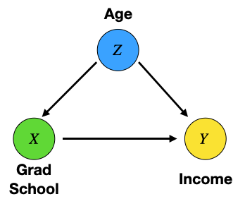
Causal models were introduced in the previous series on causality. A simple causal model can be represented by something called a Directed Acyclic Graph (DAG), which depicts the causal connections between variables via dots and arrows, where A → B represents A causes B.
We saw an example DAG in the last post of this series which looked something like the image below. Notice we don’t have (or need) the details of the connections (i.e. the functional relationships between variables), only what causes what.
Step 2 — Evaluate the Markov Condition
Once we have a DAG in hand, we can evaluate a condition that guarantees identifiability. This is called the Markov Condition, and if satisfied, causal effects are identifiable. Meaning we can compute Formula 2 from observational data (no RCT needed!).
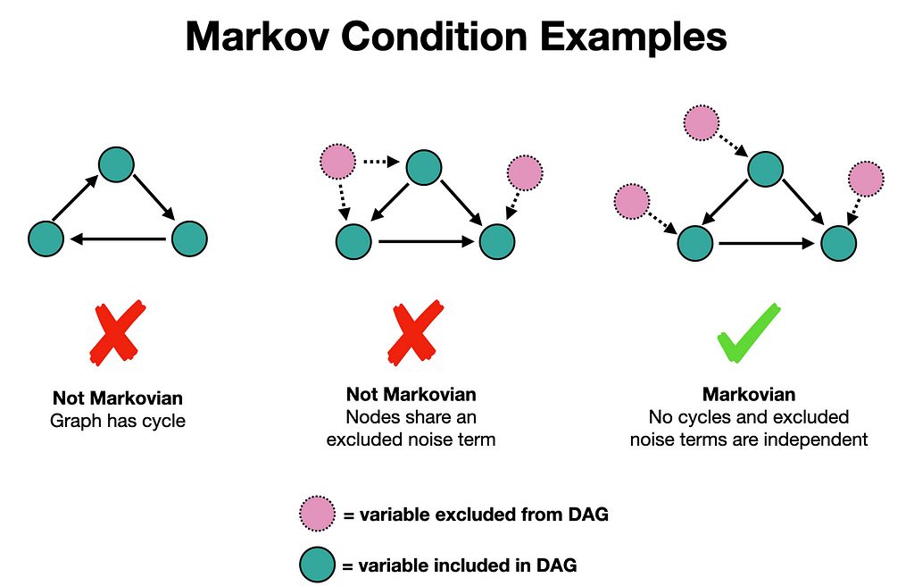
The Markov Condition has 2-parts. One, the graph must be acyclic, which is true of all DAGs (that’s what the “A” stands for). And two, all noise terms are jointly independent. What this 2nd point means is that there are no variables excluded from the DAG that simultaneously cause any 2 variables. Some examples of when this is satisfied/violated are given below.
Step 3 — Translate observations into interventions
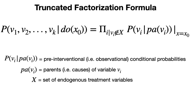
If we confirmed our DAG is Markovian (i.e. satisfies the Markov condition), we can express any interventional distribution via observational ones using the Truncated Factorization Formula given below.
To isolate treatment and outcome variables on the LHS distribution, we can sum over the covariates (i.e. all the other variables). For example, in the simple DAG from the last blog, the process would go as follows.
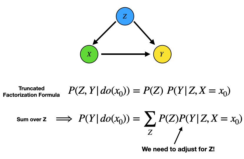
As we can see from the example above, for the given DAG we must adjust for the covariate Z. This is what we did (intuitively) back in the post on causal inference. However, here we derived this result from the truncated factorization formula, rather than relying on intuition.
This 3-step process gives us systematic way to calculate causal effects from observational data. The key that enables us to do this is a causal model that satisfies the Markov condition. We can take this process a step further and use it to deal with the problem of unmeasured confounders.
Coping with Unmeasured Confounders
A problem in data collection is variables are sometimes difficult or even impossible to measure. This raises the issue of unmeasured confounders, meaning variables that bias our causal effect estimate which we do not have data for. Again lucky for us, this Structural Causal Framework has a solution for this problem.
We explore the problem of unmeasured confounders via an example (taken) from the introduction by Pearl [1]. Suppose we have the following Markovian causal model.
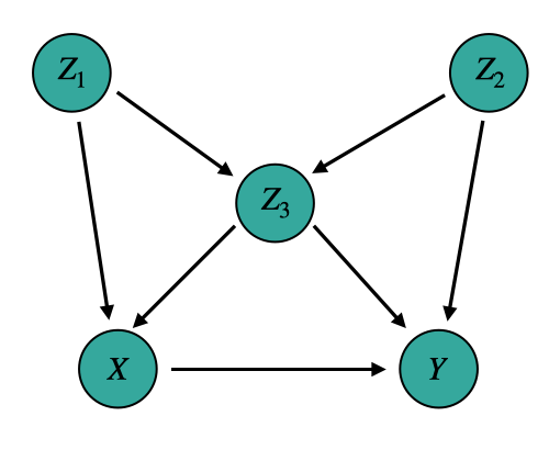
Then, like we did before, we can write down the interventional distribution P(Y | do(X=x0)) via the Truncated Factorization Formula and summing over covariates. The algebra is given in the below image.
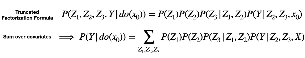
But now suppose Z_2 is hard (or impossible) to measure. How can we compute the estimation above with our data? This is indeed possible and the result is given below.
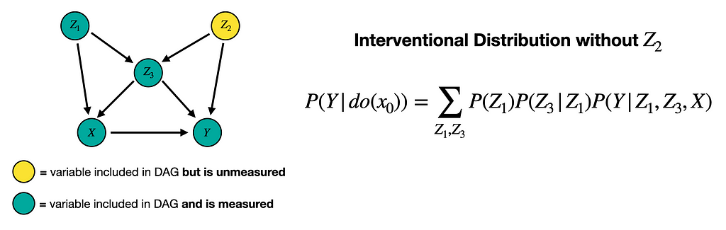
While this final step may have seemed like magic, it comes from the following equation.
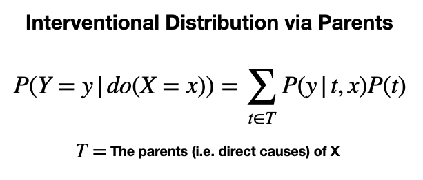
The key point here is we only need to measure the parents of X to estimate its causal effects. What makes this expression valid is the Markov condition, which requires that any variable (when conditioned on its parents) is independent of its non-descendent.
In other words, by conditioning on Z_1 and Z_3, we block that statistical dependence between X and Z_3. In next blog of this series, we will explore other possible reductions to the truncated factorization formula.
How to use this with Propensity Scores
Going back to the last article of this series, we can use what we have learned here to improve our estimates of causal effects via Propensity Scores. To generate a propensity score, we take a set of subject characteristics (i.e. covariates) and use them to predict treatment status via, for example, logistic regression [2]. However, choosing the right covariates is not a trivial step.
One way we can overcome this challenge is by including only the parents of X in the propensity score model. Therefore, if we take the time to write down a causal model for our problem, we can pick out the covariates in a straightforward way. For example, in the DAG above we would only include Z_1 and Z_3 in our propensity score model, even if Z_2 is measured.
Alternative Covariate Selection
While needing only to account for the direct causes of X is a powerful insight, what if the parents of X are unmeasured?
This motivates seeking alternative covariates with which to express our interventional distribution. In the next post of this series will do exactly this and discuss causal effects via graphical models.
Resources
More on Causality: Causality: Intro | Causal Inference | Causal Discovery | Causal Effects | Propensity Score
Connect: My website | Book a call | Message me
Socials: YouTube | LinkedIn | Twitter | Tik Tok | Instagram| Pinterest
Support: Buy me a coffee ☕️
Join Medium with my referral link - Shawhin Talebi
[1] An Introduction to Causal Inference by Judea Pearl
[2] An Introduction to Propensity Score Methods for Reducing the Effects of Confounding in Observational Studies by Peter C. Austin
Causal Effects via the Do-operator was originally published in Towards Data Science on Medium, where people are continuing the conversation by highlighting and responding to this story.
from Towards Data Science - Medium https://ift.tt/C5G9gpY
via RiYo Analytics


No comments