https://ift.tt/NXEVOzZ Everything you need to know about Stereo Geometry The Need for Multiple Views In the pin-hole model of a camera, ...
Everything you need to know about Stereo Geometry
The Need for Multiple Views
In the pin-hole model of a camera, light rays reflect off of an object and hit the film to form an image. So all the points that lie along the same ray will correspond to a single point in the image.
Hence given a point in the image, it’s impossible to pin-point its exact location in the world i.e, we cannot recover depth from a single image.
We cannot recover structure from an image as well. An example of this is shadow art where the artist makes beautiful shadows using hand gestures. There’s no way we can say anything about the gesture by only looking at the shadow.
In this article we’ll learn to deal with such ambiguities using two views.
The Epipolar Constraint
Suppose I give you two images captured from different views. I show a point in one of the image and ask you to find it in the other image. How would you do it? Here’s an idea: you could take a small patch around the point in the image and slide it across the other image and see where it matches the most.
However, once you look at the geometry, you’d realise you don’t need to scan the entire image as the point is bound to lie on a line as shown in the below figure.
The intuition is that in the real world the point can lie anywhere on the line joining its projection and the camera center. So we can reason that the projection of this point in the other image can lie anywhere on the projected line. This projected line is called the epipolar line. So now our search space reduces to this line. This is called the epipolar constraint.
In this article we’ll discuss how to solve for the epipolar line algebraically. Before that let’s get familiarised with the key definitions in epipolar geometry.
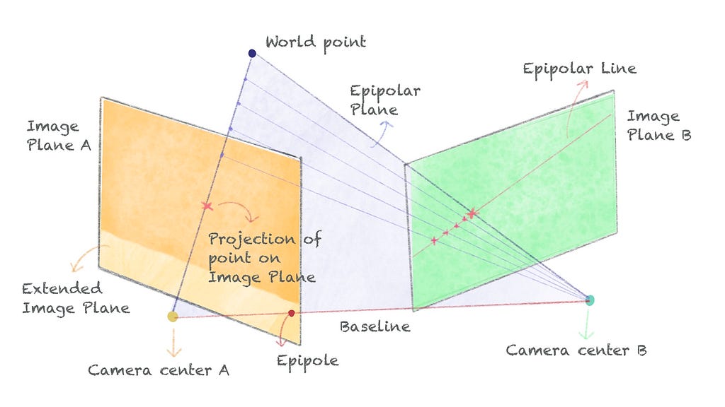
Key Terms
- Baseline: The line joining the two camera centers.
- Epipolar Line: The line along which the projected point lies. Epipolar lines come in pairs, each for an image.
- Epipolar Plane: The plane containing the baseline and a point in the world. The Epipolar plane intersects the image planes at their epipolar lines.
- Epipole: The point where the baseline intersects the image plane. All the epipolar lines corresponding to different points intersect at the epipole. Why? We saw the epipolar plane intersects the image plane at the epipolar line. Now, every epipolar plane corresponding to different points will have the baseline in common. Since the epipole is where the baseline meets the image plane, it means all the epipolar lines will have epipole as the common point. In other words, all the epipolar lines intersect at the epipole. Also, the epipole needn’t lie within the image, it can lie on the extended image plane.
Camera Matrices
In this section we’ll review homogeneous coordinates and camera matrices which we’ll be using going forward. If you’re already familiar with them or you’ve read my previous articles on camera calibration, you can skip this section.
Homogeneous Coordinates
Consider a point (u, v). To represent it in its homogeneous form, we simply add another dimension like so: (u, v, 1). The reason for this representation is because translation and perspective projection become linear operations in the homogeneous space; meaning, they can be computed through a matrix multiplication in one go. We’ll look at the homogeneous transformation matrix in detail in the later part of this article.
A key property of the homogeneous coordinates are they are scale invariant; meaning, (kx, ky, k) and (x, y, 1) represent the same point where k≠0 and k ∈ R. To convert from homogeneous to euclidean representation, we simply divide by the last coordinate like so:

If you think about it, a line from origin through the point [x, y, 1] also has the form k[x, y, 1]. So we can say a point in the image space is represented as a ray in the homogeneous space.
Homogeneous representation of a line: Consider the familiar equation ax + by + c = 0. We know that it represents an equation of a line passing through the point (x, y). Now, this equation can also be represented as l⊺p=0 where l is (a, b, c), l⊺ is the transpose of l, and p is (x, y, 1). p is essentially the homogeneous representation of the point (x, y).
Now, l is scale invariant because the equation l⊺p=0 doesn’t change if you multiply with a constant. Hence we can say l is the homogeneous representation of a line.
To summarize, given a homogeneous point p, the equation l⊺p=0 (or p⊺l=0) signifies that p lies on the line l. Keep this in mind as we’ll revisit it when discussing the essential matrix.
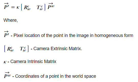
Camera Extrinsic Matrix
A camera extrinsic matrix is a change of basis matrix that converts the coordinates of a point from world coordinate system to camera coordinate system. It lets us view the world from the camera perspective. It’s a combination of rotation matrix and translation matrix — the rotation matrix orients the camera and the translation matrix moves the camera. The equation can be represented as:
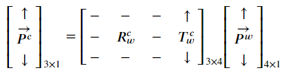
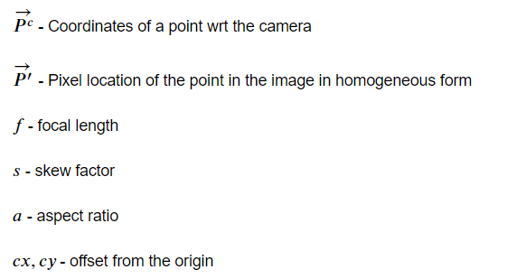
Here the notations are as follows:
For more details on the camera extrinsic matrix, please check my other article here.
Camera Intrinsic Matrix
Once we get the coordinates of the points wrt the camera using the camera extrinsic matrix, the next step is to project them onto the image plane of the camera to form an image. This is the job of the camera intrinsic matrix. The camera intrinsic matrix has been discussed in-depth in my other article, but to summarize, the camera intrinsic matrix projects the points whose coordinates are given wrt the camera onto the image plane of the camera. It essentially encodes the properties of camera’s film. The equation is shown below:
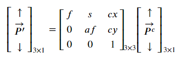
The notations are:
The Image Formation Pipeline
So, given a point and a camera in the world, we represent the point in its homogeneous form and multiply with the extrinsic matrix to get its coordinates wrt the camera frame. Then we multiply with the intrinsic matrix to get its projection on the image plane of the camera. Finally, we convert back to euclidean coordinates to get the point’s pixel location in the image. This is the image formation pipeline and is shown below:
The Essential Matrix
Alright, we’ll now discuss the foundation of stereo geometry — the essential matrix. let’s derive it and see what it does.
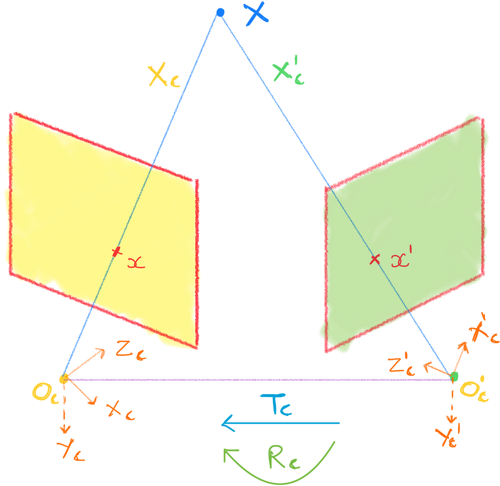
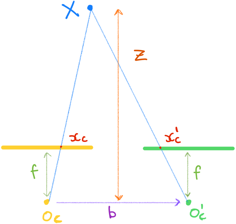
Consider a calibrated system where we know the relative position and orientation of the two cameras. Let the camera centers be denoted as Oc and Oc′. Let X be a point in the world. Let’s represent the coordinates of X wrt camera frame Oc as Xc and wrt Oc′ as Xc′. Let Rc and Tc be the rotation and translation change of basis matrices from Oc to Oc′. It means given the coordinates of X wrt Oc, we can find them wrt Oc′ as:

The cross product matrix
Let’s take a small detour and talk about the vector cross product. The cross product of two vectors a, b will be a vector perpendicular to both of them and is represented by a×b = [-a3b2 + a2b3, a3b1-a1b3, -a2b1 + a1b2] where a = [a1, a2, a3] and b=[b1, b2, b3].
We can represent the same in matrix form as:

This matrix form of cross product is represented as [a×]b where [a×] is a 3 × 3 matrix and b is a 3 × 1 vector.


Now, the cross product of a vector with itself is zero. i.e a×a = [a×]a = 0. So we can say [a×] is a skew-symmetric matrix with rank 2.
Back to our equation:
Taking the cross product on both sides with the vector Tc we get:

Tc × Tc = 0. Next, we take the dot product on both sides with the vector Xc′:

Now, the vector 𝑇 ×Xc′ is perpendicular to Xc′. Hence, Xc′.(𝑇 × Xc′) = 0.

Now, Tc and RcXc are both 3 dimensional vectors. So we can represent their cross product in matrix form as:

Finally we can represent the equation as:


The matrix E is called the Essential Matrix and it relates the coordinates of a point wrt two different camera frames.
Finding the Epipolar Lines
Now, how can we find the epipolar lines using the essential matrix? let’s take a deeper look at the equation.

Here Xc is the coordinates of the point X wrt the camera frame Oc. It means we can represent any point along the line joining X and Oc wrt Oc as 𝛼Xc where 𝛼 is some constant. Now, if we substitute Xc with 𝛼Xc in the equation, it’d still satisfy.

Similary we can substitute Xc′ with 𝛽Xc′ where 𝛽 is some constant and the equation remains the same.
So we can say the essential matrix equation is satisfied by any two points that lie along the projective rays joining the point and their respective camera centers, where the coordinates of the points are represented wrt their camera frames.
Let x𝑐 and xc′ be the projections of the point X on the image planes of cameras Oc and O𝑐′. They must satisfy the essential matrix equation as they lie along the projective rays. So we can write:

Now xc is a 3 × 1 vector and E is a 3 × 3 matrix so their product will be a 3 × 1 vector. let’s represent it by l:

This equation should look familiar to you. As discussed in the previous section, this equation represents the homogeneous point xc′ lies on the line l. We can say l is the epipolar line corresponding to the point xc, and xc′ lies on this line. This is the mathematical form of the epipolar constraint.

Similarly, as shown in the above equation, l′ is the epipolar line corresponding to the point xc′, and xc lies on this line.
So given the projection of a point in one view, we multiply it with the essential matrix to obtain the epipolar line on which the projection of the point in the other view lies.
This is a bit tricky to implement in practice, but I’ve got you covered.
Python Example
All the code for this article can be found in this repository. The instructions to setup the environment can also be found there. Here’s the notebook for this section. Just skim through it now, I’ll provide a step-by-step breakdown below.
Setting up the Environment
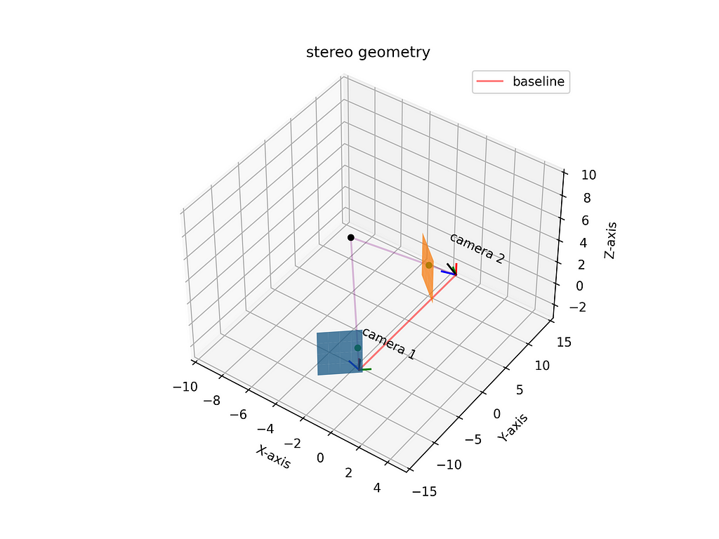
First we define extrinsic parameters for both the cameras such that they’re placed some distance apart at an angle. The extrinsic parameters include camera’s position and orientation.
Next we define intrinsic parameters which dictate the formation of the image. Here we’ve the defined the size of the image plane and the focal length, which essentially is a measure of how far the image plane is from the camera center.
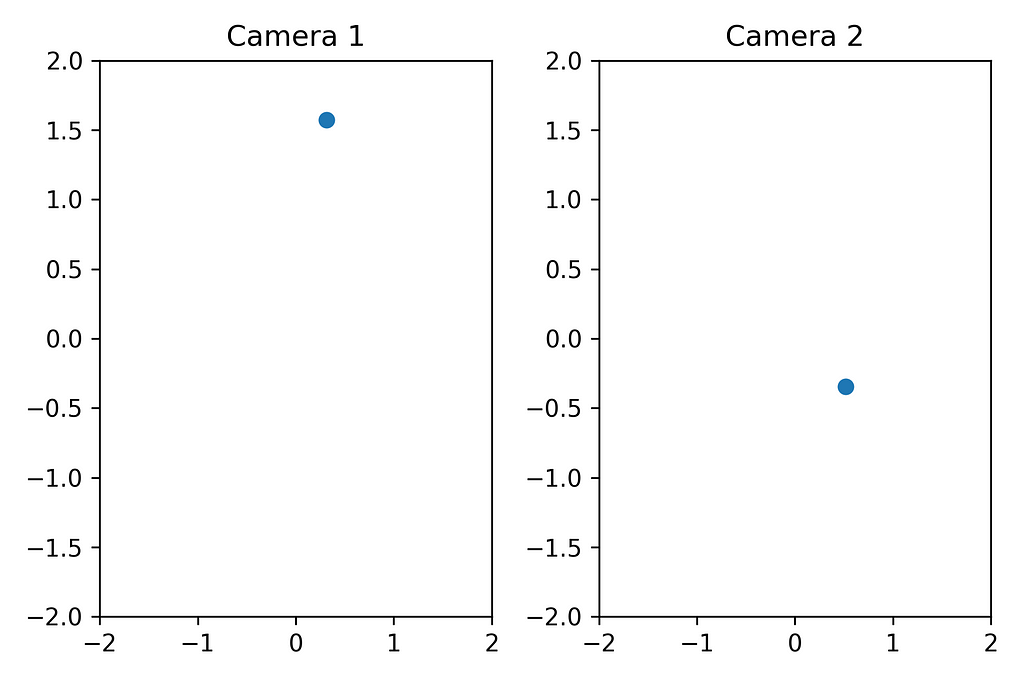
We also define a point in the world such that it’s captured by both the cameras. In this example, we’ll find the epipolar lines for the projections of this point.
The images captured in the both the views are shown below:
Computing the Essential Matrix
To find the essential matrix, we need to find the relative geometry between the two cameras such that given the coordinates of a point wrt camera 1, we should be able to find its coordinates wrt camera 2.
Now, we know the camera extrinsic matrix is a change of basis matrix from the world coordinate system to the camera coordinate system. Using this information, the change of basis matrix from camera 1 to camera 2 can be computed as follows:
change of basis matrix from camera 1 to camera 2 = (change of basis matrix from world to camera 2) × (change of basis matrix from camera 1 to world)
⟹ change of basis matrix from camera 1 to camera 2 = (change of basis matrix from world to camera 2) × (inverse of change of basis matrix from world to camera 1)
⟹ change of basis matrix from camera 1 to camera 2 = (Extrinsic Matrix of camera 2) × (inverse of Extrinsic matrix of camera 1)
Once we obtain this change of basis matrix, we can extract the relative orientation and offset of the cameras. The first 3 columns of this 3 × 4 matrix will give the orientation Rc, and the last column will give the offset Tc.

We then compute the cross product matrix of Tc and multiply it with Rc to obtain the essential matrix.

As a sanity check, we can validate the essential matrix equation.

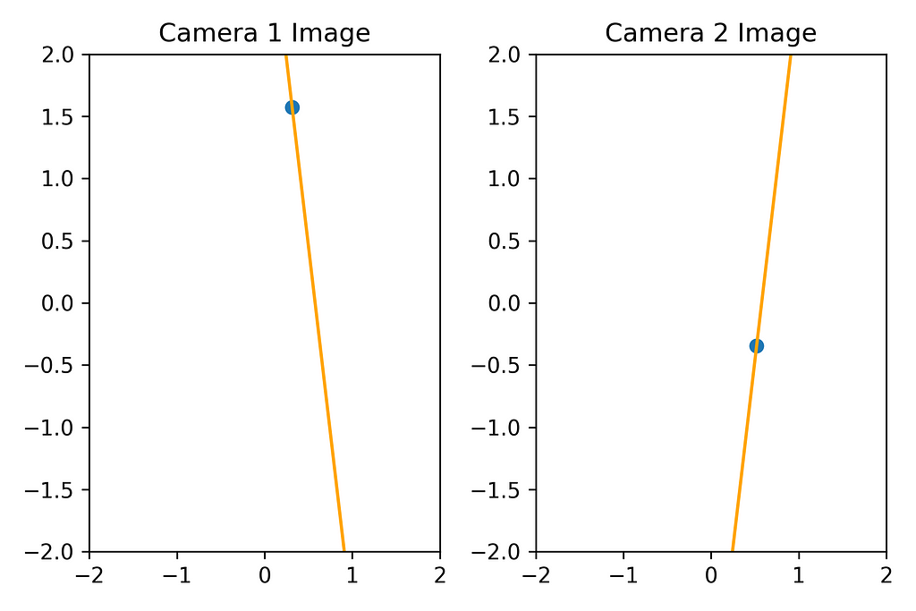
Plotting the Epipolar lines
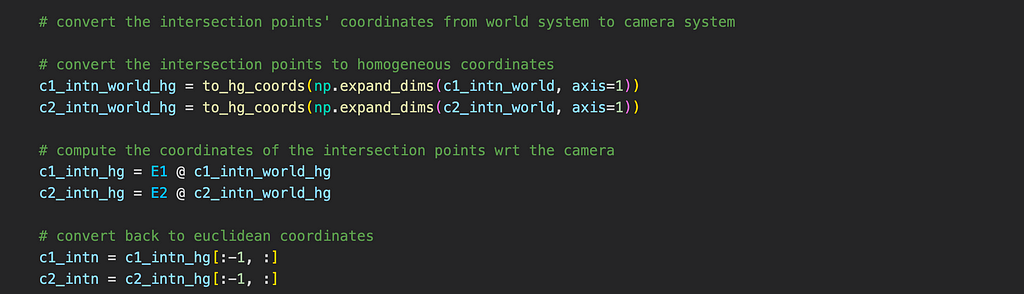
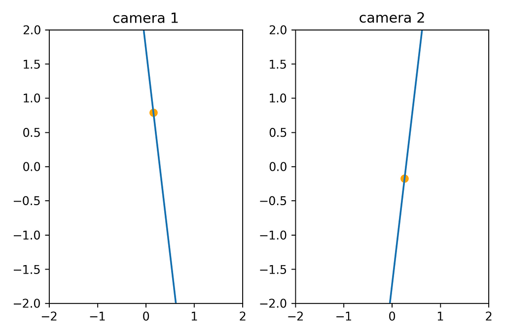
To find the epipolar lines, we first need to find the projections of the point on the image planes of the cameras. In this example, I’ve manually plotted these points through trial and error, but we’ll see a better way to find them in a later section.
Once we find these points, we multiply them with their respective extrinsic matrices to get the coordinates wrt camera frames. Then we plug them in the essential matrix equation and find the corresponding epipolar lines.
For example, if we know the projection point in camera 1, we multiply it with the essential matrix to get the epipolar line in camera 2. We then plot this line in the 2D image space. To verify the projection point in camera 2 lies on this line, we convert it to euclidean coordinates and plot it in the same space. We repeat the same process for the other camera.
The projection points and their corresponding epipolar lines in the image space are shown below:
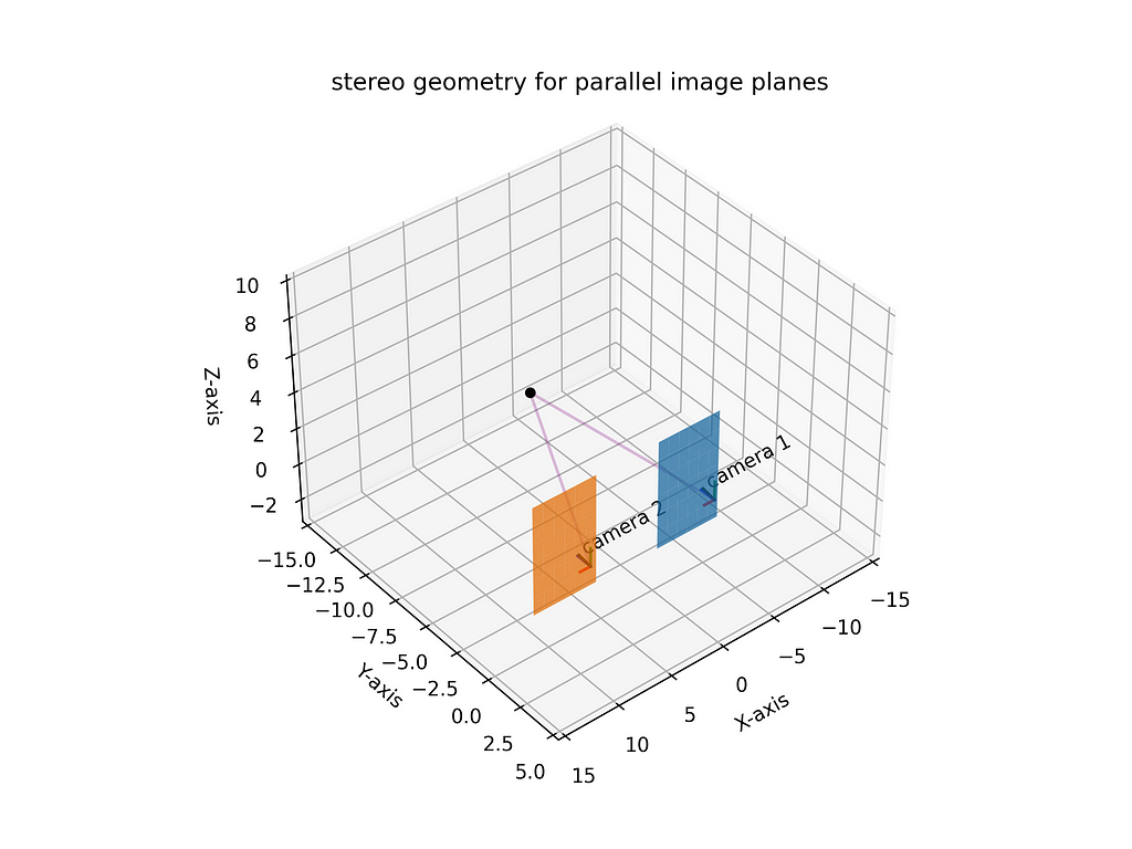
Parallel Image Planes
What happens if the image planes are parallel to each other? In the above system we have two cameras with their optical axes parallel to each other along the Y-axis. Let’s assume the camera centers are on the X-axis and are b distance apart.
Since the cameras are parallel, there is no relative rotation between them. So Rc will be an identity matrix and Tc will be equal to [-b, 0, 0] (-ve sign because Tc represents a change of basis operation which is the inverse of the transformation operation). So we can compute the essential matrix as:


Let x𝑐 and xc′ be the projections of the point X on the image planes of cameras Oc and O𝑐′. If we assume the focal length of both the cameras is f, we can write xc = [x, y, f] and xc′ = [x′, y′, f]. We can plug them in the essential matrix equation like so:


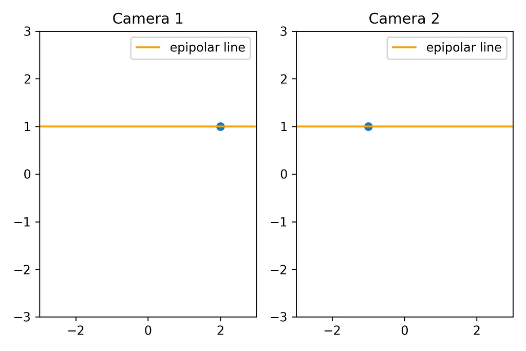
We can see the epipolar lines have the same Y-coordinate, meaning they’re parallel along the X-axis. Hence we can say if two cameras are parallel to each other, their epipolar lines will also be parallel in the image space.
This is illustrated below:
The code for this section can be found here.
If the cameras are parallel along the Y-axis, the epipolar lines in the images would be horizontal; if they’re parallel along the X-axis, the epipolar lines would be vertical.
The Fundamental Matrix
In real life, we seldom have information about the location of points in the world. However, we can find their location in the image. So we need to modify the essential matrix equation to account for the image location of points.
Now, given a point in the world wrt the camera frame, the intrinsic matrix is responsible to project it onto the image plane of the camera.

We can send κ to the other side and rewrite the equation as:

So, given a point in the image, we represent it in homogeneous form and multiply with the inverse of intrinsic matrix to get the homogeneous representation of the point in the world.
Now, we cannot pin-point the exact location of the point in the world from the image because homogeneous coordinates are scale invariant and the point can lie anywhere on the ray.
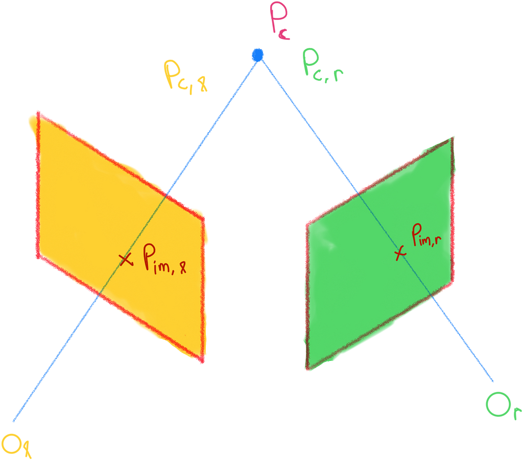
Consider two camera frames l and r, and a point Pc that projects on both the image planes. The essential matrix equation here is:

In this equation we can substitute the homogeneous image coordinates like so:


This is called the fundamental matrix equation.
The essential matrix relates coordinates of the same point in two different views, while the fundamental matrix relates them in two different images.
In the previous example, we can compute the fundamental matrix and plot the epipolar lines like so:

If you observe, the epipolar lines look exactly the same as before, however, this time they were computed directly from the image coordinates using the fundamental matrix equation.
Computing the Fundamental Matrix from Point Correspondences
We rarely work with a calibrated system in the real world. However, since the fundamental matrix relates image points directly, we can still find it without any knowledge of the world and the cameras. Here’s how.
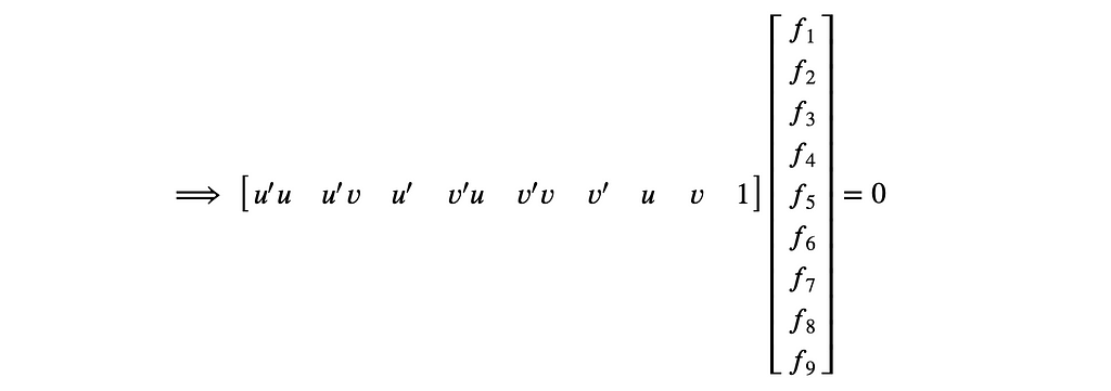
Let (u, v) and (u′, v′) represent the same point in two different images. We can represent them in homogeneous form and plug in the fundamental matrix equation:

Here f1, f2, … represent the unknown parameters of the fundamental matrix. The above equation represents a homogenous system, and I’ve discussed them in depth in my other article here. However, I’ll discuss the intuition again here.
The first step is to rewrite the equation as:
A reason to rewrite this way is we can stack many point correspondences in the same equation like so:
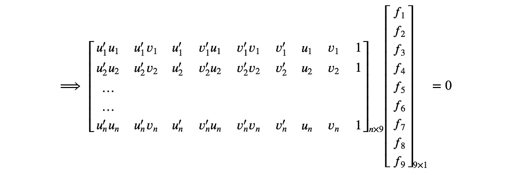
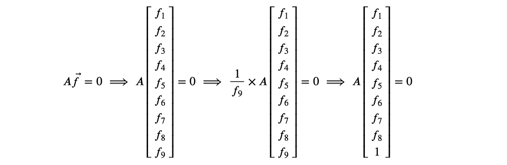
This equation can be represented in matrix notation as Af ⃗= 0, where A is the point correspondence matrix and vector f ⃗ is the flattened fundamental matrix. Now, f ⃗ can be made into a unit vector by dividing both sides of the equation with its magnitude |f ⃗|.
A solution to equations of type Ax ⃗= 0 subject to constraint |x⃗|=1 can be found by computing the minimum value of |Ax⃗|.
In my other article, I’ve discussed that |𝐴𝑥⃗| will be minimum if the unit vector 𝑥⃗ is along the smallest eigenvector of 𝐴⊺𝐴.
This is called the linear least square estimate.
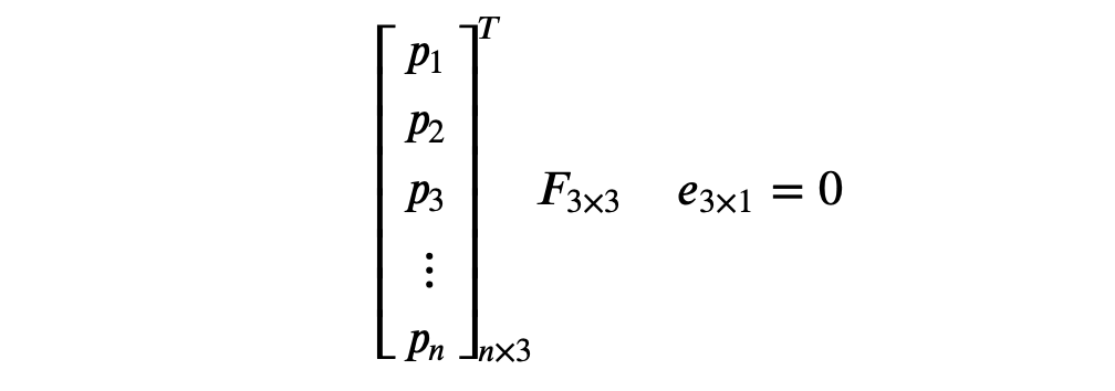
The Eight Point Algorithm
The idea is to find point correspondences between the images and compute matrix 𝐴. Then the fundamental matrix can be found by computing the smallest eigenvector of 𝐴⊺𝐴 and reshaping it as a 3 x 3 matrix.
How many points do we require at minimum to compute f ? Now, f has 9 unknowns so you’d say we need 9 equations or 9 points to solve for it. But if you observe, f is scale invariant, meaning we can multiply f with any constant and the equation Af ⃗= 0 is still satisfied. So we can divide f with one of its values like so:
Now see there are 8 unknowns to solve for and we only need 8 points at minimum.
There’s another thing we need to account for. You see, the 3 ×3 fundamental matrix F has rank = 2. We’ll not discuss the proof here, but this has to do with the fact that the cross-product matrix has rank 2.
So to account for this, we perform singular value decomposition on the matrix F, make its last singular value zero, and recombine again.
The code for the eight point algorithm is shown below:
Normalized Eight Point Algorithm
Modern images have a high resolution of ~ 4000 — 6000 px. This causes a lot of variance in the point correspondences which might break the algorithm. So to account for this, we normalize the points before plugging them into the eight point algorithm.
The idea is for each image we compute the centroid (mean) of the point correspondences and subtract it from each of them. Next we scale them such that the distance from the centroid (variance) is √2 as shown below:

Next we create a matrix that performs the above transformation and use it to transform the points as shown in the code below:
Finding Epipole
We know the epipole is a point where all the epipolar lines in an image meet. Mathematically it can be represented as:

Where l1, l2, … are the epipolar lines and e is the epipole. This can be represented in matrix form as:
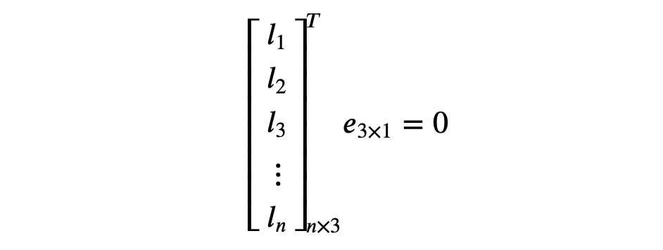
Now this looks like a system of homogeneous equations. So to find the epipole, we can find a solution to Le⃗ = 0 using the linear least square estimate as discussed in the previous section.
But wait, the epipolar lines can be computed from the fundamental matrix. So we can rewrite the equation as:
Now to find the solution to this equation, we simply compute the linear least square estimate of F which is its last singular value.
The code to compute epipole is shown below:
To find the epipole for the other image, we find the linear least square estimate of F transpose.
Python Example
Alright, let’s see the fundamental matrix in action.
The notebook can be found here. Let’s walk through it.
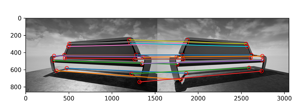
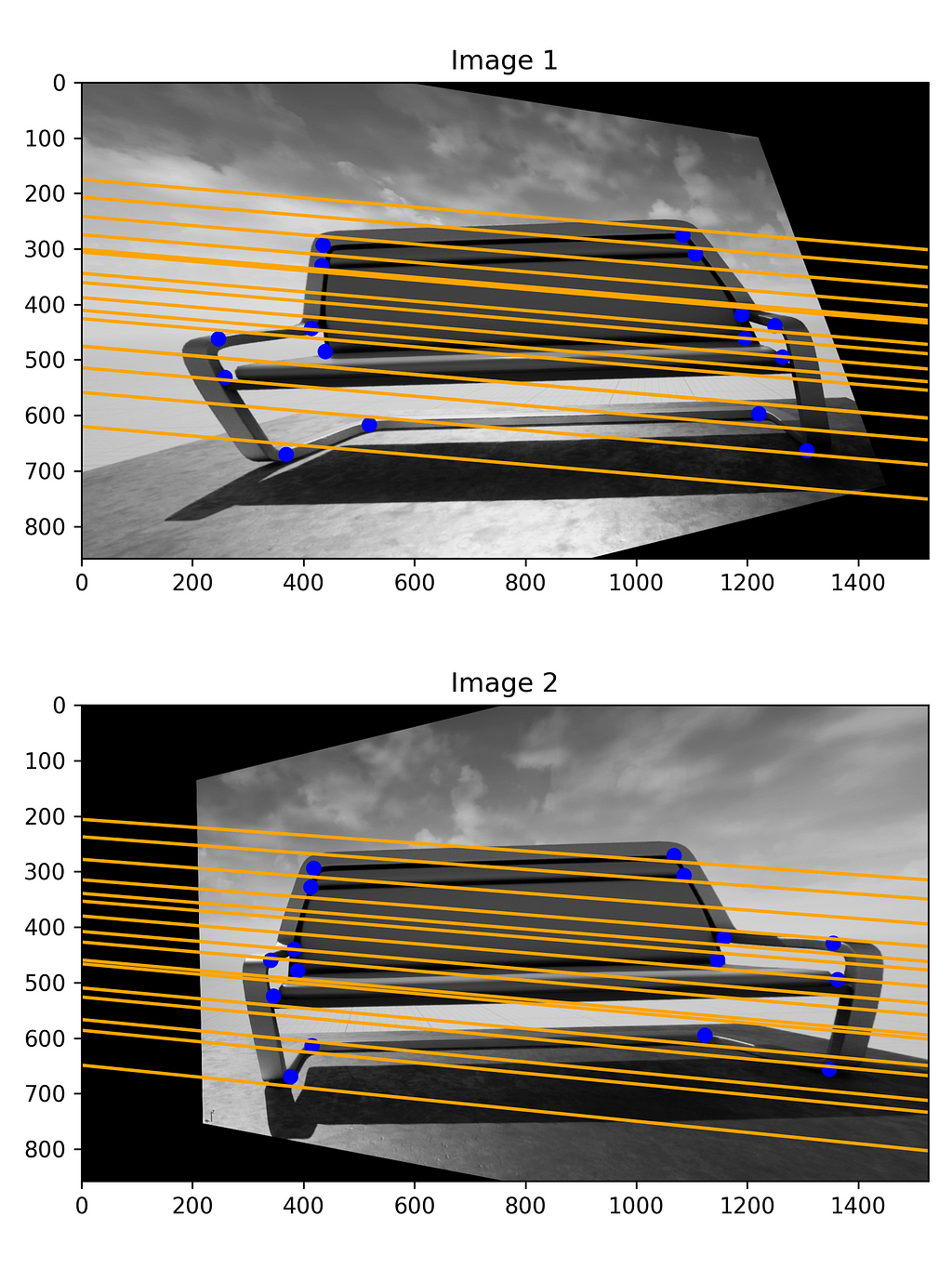
First we need two images of the same object. So I opened my unreal editor, placed two cameras looking at the same object, and took screenshots.


Next, we need point correspondences or matches between the two images. Here I’ve manually labelled them, but in the real world we can use algorithms like SIFT to automatically compute them.
Alright, now we can compute the fundamental matrix from the points using the normalized eight point algorithm.

We can also validate the fundamental matrix equation using the computed matrix.

Let’s plot the epipolar lines for both the images.
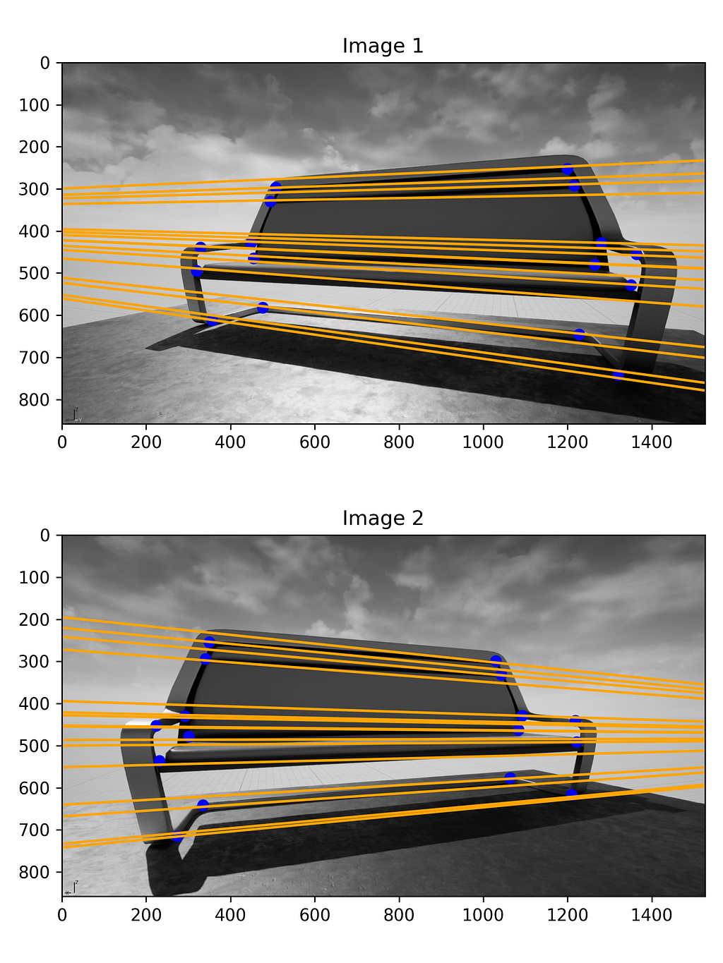
We can see the epipolar lines corresponding to one image pass through the points in the other image.
Next let’s find and plot the epipoles.

The fundamental matrix equation also holds true for epipoles since they’re also points in the image plane.

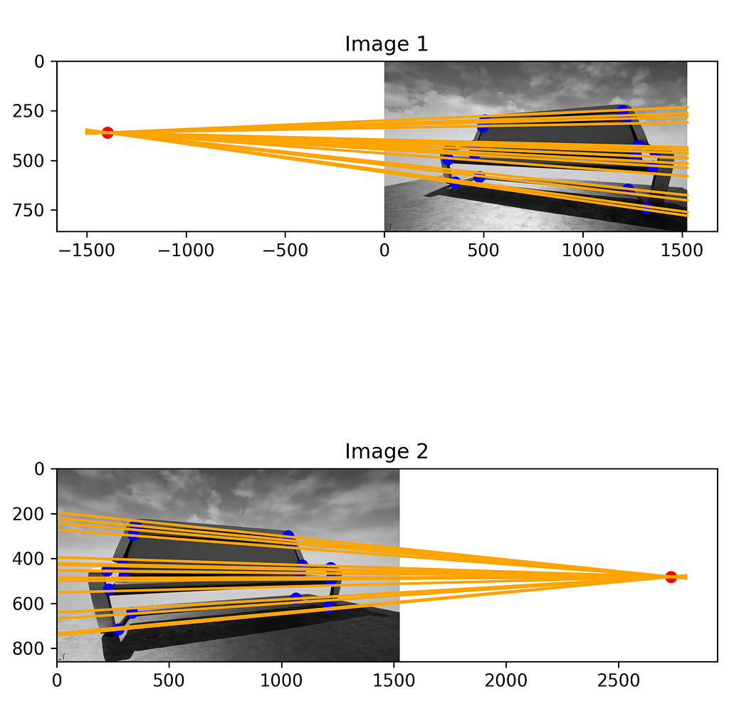
We can see here the epipoles lie way beyond the image, and all the epipolar lines intersect at them.
Stereo Rectification
It’s easy to work with images with parallel image planes as the epipolar lines are parallel. However, it’s possible to make them parallel by warping them strategically. This process is called stereo rectification. Let’s see how to do it.
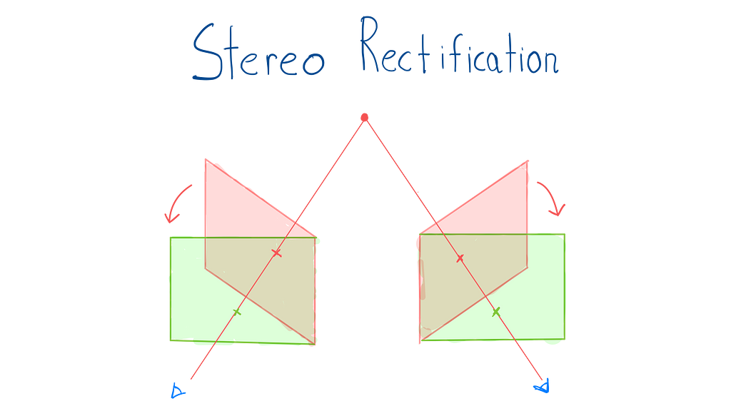
For parallel images, the epipoles lie at infinity along the horizontal axis. So the first step is to create transformation matrices to move a point to infinity.
We’d need three transformation matrices: one to rotate a point to the horizontal axis, one to shift the point to infinity, and one to translate the origin to center. Let’s look at each of them.
Rotating a point to horizontal axis
Given a point that makes an angle θ with the X-axis, we create a rotation matrix that rotates it by -θ and brings it back to the X-axis as shown below:
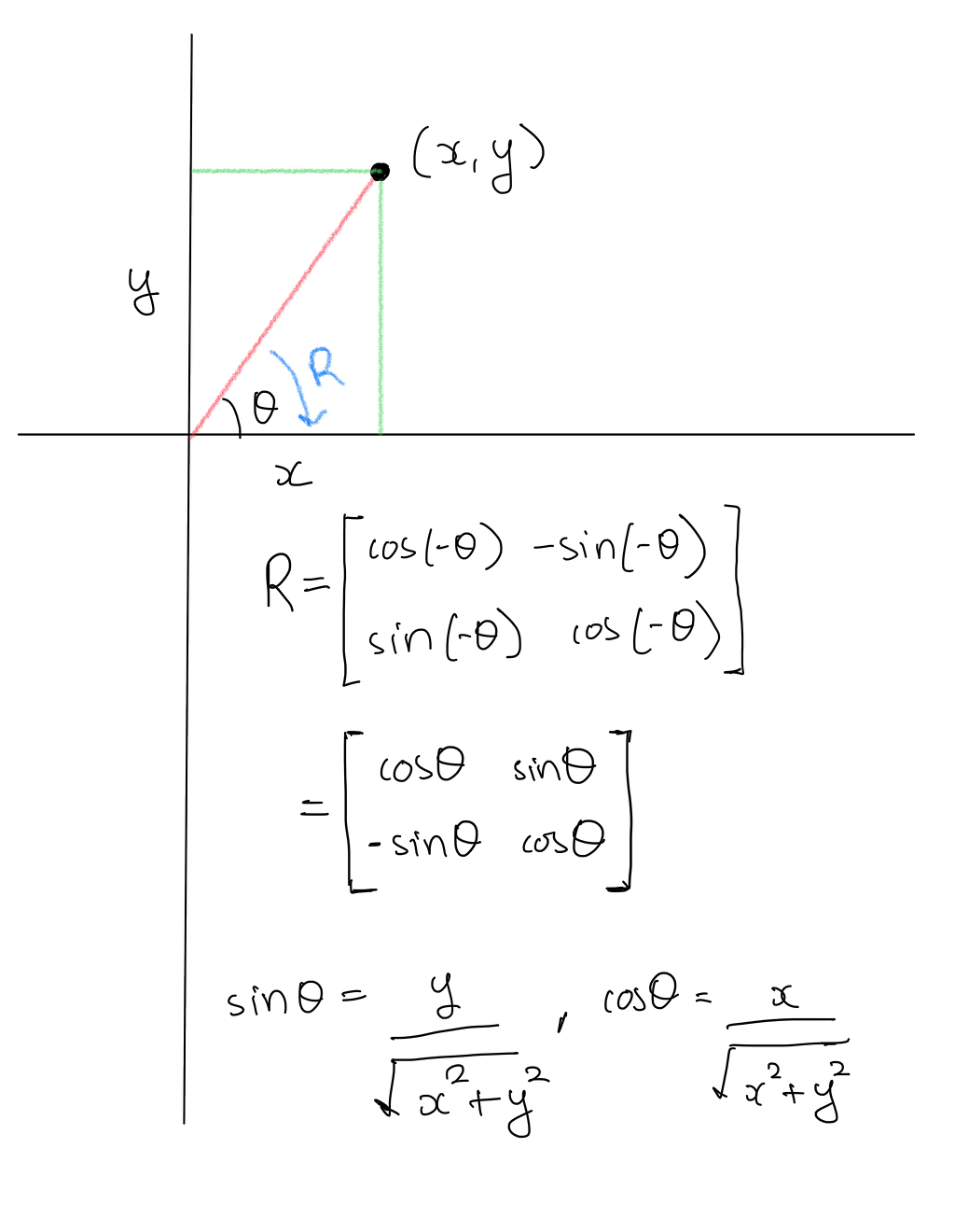
Note: the signs will be reversed if the point lies on the other side of X-axis.
Since we’re dealing with homogeneous coordinates, we need to account for the additional dimension.
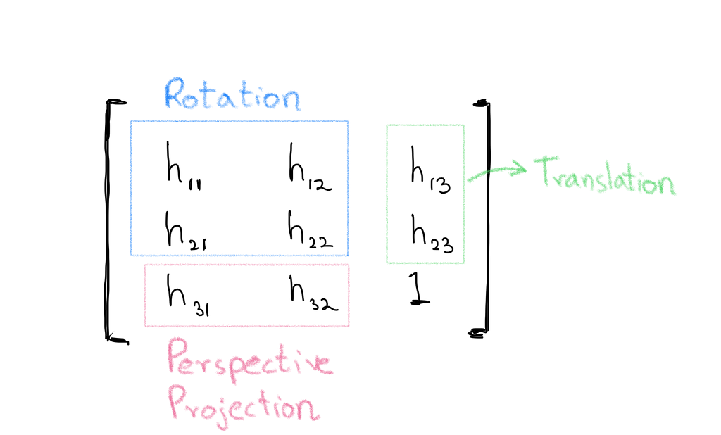
The general transformation matrix for homogeneous coordinates, also called the homography matrix, is shown below:
So the matrix needed to rotate a homogeneous coordinate back to X-axis is:

Shifting the point to infinity
Next we need to shift the point to infinity. A point at infinity is represented as (∞, 0) or (-∞, 0). The same can be represented in homogeneous coordinates as (x, 0, 0) as shown below:

So given a point lying on the X-axis represented in its homogeneous form as (x, 0, 1), we need a matrix that transforms it to (x, 0, 0).
The following matrix does the job:

Moving the origin to center
By default Python assumes the image’s origin is located at the top left corner, so we need to create a translation matrix to move the origin to center.

After applying the transformations, we can shift it back to its original place.
Warping Images
So the overall transformation matrix combining the above matrices is given by:

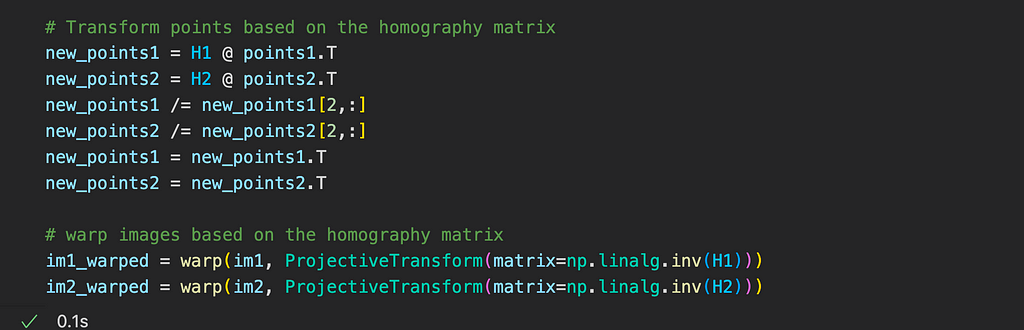
The idea is we transform the points with the above matrix, and then to “undo” the effect, we warp the entire image with the inverse of the matrix.
Using this technique we can warp one image. Now, how to warp the other image? Richard Hartley in his paper argues that to get best results, both the stereo images need to be aligned, meaning the distance between the transformed point correspondences should be minimum.
So the matching homography matrix H1 can be found by minimizing the sum of squared distances between the transformed point correspondences:

We’ll not go through the proof of computing H1 here, but I’ve linked it in the references section at the end for the interested reader.
The code snippet for computing H1 and H2 is shown below:
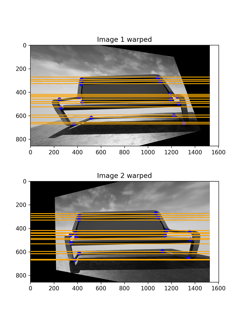
Alright, let’s rectify the images in our example.
Once we compute the homography matrices, the images can be warped using their inverses as shown below:
We now have rectified images with parallel image planes, so the epipolar lines are simply horizontal lines passing through the points.
An Empirical Observation
If I compute the fundamental matrix and epipolar lines for the warped images using the normalized eight point algorithm, the result is not accurate as can be seen below:
I don’t know the exact reason but I think the algorithm is breaking because the epipoles are at infinity. Let me know what you think.
The rectified images now can be used for various downstream tasks like disparity estimation, template matching, etc.
Conclusion
Alright, we’ve reached the end. In this article we’ve looked at techniques to deal with images captured from two views. We’ve also seen how certain ambiguities like depth can be estimated from two images using stereo rectification. If we’ve multiple views, we can also estimate the structure of the scene using a technique called Structure from Motion.
Moreover, with the recent advances in deep learning, all of these ambiguities can be estimated from a single image. We’ll perhaps discuss them in future articles.
I hope you’ve enjoyed the article.
Let’s connect. You can also reach me on LinkedIn and Twitter. Let me know if you’ve any doubts or suggestions.
References
- cs231a Notes
- https://github.com/chizhang529/cs231a
- Theory and Practice of Stereo Rectification by Richard Hartley
Image Credits
All the images displayed in this article are by the author.
A Comprehensive Tutorial on Stereo Geometry and Stereo Rectification with Python was originally published in Towards Data Science on Medium, where people are continuing the conversation by highlighting and responding to this story.
from Towards Data Science - Medium https://ift.tt/QYtTavX
via RiYo Analytics


ليست هناك تعليقات