https://ift.tt/s3Z0YwV When training a deep neural network, it’s often troublesome to achieve the same performances on both the training an...
When training a deep neural network, it’s often troublesome to achieve the same performances on both the training and validation sets. A considerably higher error on the validation set is a clear flag for overfitting: the network has become too specialized in the training data. In this article, I provide a comprehensive guide on how to bypass this issue.

Overfitting in a Neural Network
When dealing with any machine learning application, it’s important to have a clear understanding of the bias and variance of the model. In traditional machine learning algorithms, we talk about the bias vs. variance tradeoff, which consists of the struggle when trying to minimize both the variance and the bias of a model. In order to reduce the bias of a model, i.e. reduce its error from erroneous assumptions, we need a more complex model. On the contrary, reducing the model’s variance, i.e. the sensitivity of the model in capturing the variations of the training data, implies a more simple model. It is straightforward that the bias vs. variance tradeoff, in traditional machine learning, derives from the conflict of necessitating both a more complex and a simpler model at the same time.
In the Deep Learning era there exist tools to reduce just the model’s variance without hurting the model’s bias or, on the contrary, to reduce the bias without increasing the variance. Before exploring the different techniques used to prevent the overfitting of a neural network, it’s important to clarify what high variance or high bias means.
Consider a common neural network task such as image recognition, and think over a neural network that recognizes the presence of pandas in a picture. We can confidently assess that a human can carry out this task with a near 0% error. As a consequence, this is a reasonable benchmark for the accuracy of the image recognition network. After training the neural network on the training set and evaluating its performances on both the training and validation sets, we may come up with these different results:
- train error = 20% and validation error = 22%
- train error = 1% and validation error = 15%
- train error = 0.5% and validation error = 1%
- train error = 20% and validation error = 30%
The first example is a typical instance of high bias: the error is large on both the train and validation sets. Conversely, the second example suffers from high variance, having a much lower accuracy when dealing with data the model didn’t learn from. The third result represents low variance and bias, the model can be considered valid. Finally, the fourth example shows a case of both high bias and variance: not only the training error is large when compared with the benchmark, but the validation error is also higher.
From now on, I will present several techniques of regularization, used to reduce the model’s overfitting to the training data. They are beneficial for cases 2. and 4. of the previous example.
L1 and L2 Regularization for Neural Networks
Similar to classical regression algorithms (linear, logistic, polynomial, etc.), L1 and L2 regularizations find place also for preventing overfitting in high variance neural networks. In order to keep this article short and on-point, I won’t recall how L1 and L2 regularizations work on regression algorithms, but you can check this article for additional information.
The idea behind the L1 and L2 regularization techniques is to constrain the model’s weights to be smaller or to shrink some of them to 0.
Consider the cost function J of a classical deep neural network:

The cost function J is, of course, a function of the weights and biases of each layer 1, …, L. m is the number of training examples and ℒ is the loss function.
L1 Regularization
In L1 Regularization we add the following term to the cost function J:

where the matrix norm is the sum of the absolute value of the weights for each layer 1, …, L of the network:

λ is the regularization term. It’s a hyperparameter that must be carefully tuned. λ directly controls the impact of the regularization: as λ increases, the effects on the weights shrinking are more severe.
The complete cost function under L1 Regularization becomes:

For λ=0, the effects of L1 Regularization are null. Instead, choosing a value of λ which is too big, will over-simplify the model, probably resulting in an underfitting network.
L1 Regularization can be considered as a sort of neuron selection process because it would bring to zero the weights of some hidden neurons.
L2 Regularization
In L2 Regularization, the term we add to the cost function is the following:

In this case, the regularization term is the squared norm of the weights of each network’s layer. This matrix norm is called Frobenius norm and, explicitly, it’s computed as follows:

Please note that the weight matrix relative to layer l has n^{[l]} rows and n^{[l-1]} columns.
Finally, the complete cost function under L2 Regularization becomes:

Again, λ is the regularization term and for λ=0 the effects of L2 Regularization are null.
L2 Regularization brings towards zero the values of the weights, resulting in a more simple model.
How do L1 and L2 Regularization reduce overfitting?
L1 and L2 Regularization techniques have positive effects on overfitting to the training data for two reasons:
- the weights of some hidden units become closer (or equal) to 0. As a consequence, their effect is weakened and the resulting network is simpler because it’s closer to a smaller network. As stated in the introduction, a simpler network is less prone to overfitting.
- for smaller weights, also the input z of the activation function of a hidden neuron becomes smaller. For values close to 0, many activation functions behave linearly.
The second reason is not trivial and deserves an expansion. Consider a hyperbolic tangent (tanh) activation function, whose graph is the following:
From the function plot we can see that if the input value x is small, the function tanh(x) behaves almost linearly. When tanh is used as the activation function of a neural network’s hidden layers, the input value is:

which for small weights w is also close to zero.
If every layer of the neural network is linear, we can prove that the whole network behaves linearly. Thus, constraining some of the hidden units to mimic linear functions, leads to a simpler network and, as a consequence, helps to prevent overfitting.
A simpler model often is not capable to capture the noise in the training data and therefore, overfitting is less frequent.
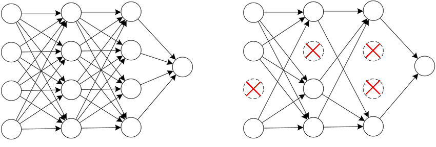
Dropout
The idea of dropout regularization is to randomly remove some nodes in the network. Before the training process, we set a probability (suppose p = 50%) for each node of the network. During the training phase, each node has a p probability to be turned off. The dropout process is random, and it is performed separately for each training example. As a consequence, each training example might be trained on a different network.
As for L2 Regularization, the result of dropout regularization is a simpler network, and a simpler network leads to a less complex model.
Dropout in practice
In this brief section, I show how to implement Dropout regularization in practice. I will go through a few simple lines of code (python). If you are only interested in the general theory of regularization, you can easily skip this section.
Suppose we have stored the activation values of the network’s layer 4 in the numpy array a4. First, we create the auxiliary vector d4:
# Set the keeping probability
keep_prob = 0.7
# Create auxiliary vector for layer 4
d4 = np.random.rand(a4.shape[0], a3.shape[1]) < keep_prob
The vector d4 has the same dimensions as a4 and contains the values True or False based on the probability keep_prob. If we set a keeping probability of 70%, that is the probability that a given hidden unit is kept, and therefore, the probability of having True value on a given element of d4.
We apply the auxiliary vector d4 to the activations a4:
# Apply the auxiliary vector d4 to the activation a4
a4 = np.multiply(a4,d4)
Finally, we need to scale the modified vector a4 by the keep_prob value:
# Scale the modified vector a4
a4 /= keep_prob
This last operation is needed to compensate for the reduction of units in the layer. Carrying out this operation during the training process allows us not to apply dropout during the test phase.
How does dropout reduce overfitting?
Dropout has the effect of temporarily transforming the network into a smaller one, and we know that smaller networks are less complex and less prone to overfitting.
Consider the network illustrated above, and focus on the first unit of the second layer. Because some of its inputs may be temporarily shut down due to dropout, the unit can’t always rely on them during the training phase. As a consequence, the hidden unit is encouraged to spread its weights across its inputs. Spreading the weights has the effect of decreasing the squared norm of the weight matrix, resulting in a sort of L2 regularization.
Setting the keeping probability is a fundamental step for an effective dropout regularization. Typically, the keeping probability is set separately for each layer of the neural network. For layers with a large weight matrix, we usually set a smaller keeping probability because, at each step, we want to conserve proportionally fewer weights with respect to smaller layers.
Other Regularization Techniques
In addition to L1/L2 regularization and dropout, there exist other regularization techniques. Two of them are data augmentation and early stopping.
From the theory, we know that training a network on more data has positive effects on reducing high variance. As getting more data is often a demanding task, data augmentation is a technique that, for some applications, allows machine learning practitioners to get more data almost for free. In computer vision, data augmentation provides larger training set by flipping, zooming, and translating the original images. In the case of digits recognition, we can also impose distortion on the images. You can check this application of data augmentation for handwritten digit recognition.
Early stopping, as the name suggests, involves stopping the training phase before the initially defined number of iterations. If we plot the cost function on both the training set and the validation set as a function of the iterations, we can experience that, for an overfitting model, the training error always keeps decreasing but the validation error might start to increase after a certain number of iterations. When the validation error stops decreasing, that is exactly the time to stop the training process. By stopping the training process earlier, we force the model to be simpler, thus reducing overfitting.
Regularization Techniques for Neural Networks was originally published in Towards Data Science on Medium, where people are continuing the conversation by highlighting and responding to this story.
from Towards Data Science - Medium https://ift.tt/VxQfNEs
via RiYo Analytics


ليست هناك تعليقات