https://ift.tt/fyH6RlF Population versus Sample: Can We Really Look at Everything? Statistical experiments in Python Photo by Ryoji Iwat...
Population versus Sample: Can We Really Look at Everything?
Statistical experiments in Python

Most of us have already learned about probability theory and statistics at school or university. What I find difficult about the subject is that while immensely useful in practical application, the theory is difficult to understand. One reason for that is that looking at some concepts introduced more closely opens up almost-philosophical questions. What is a population in statistics? Well, basically everything we want to look at. What is everything? Can we really look at everything?
The second challenge is that concepts stack up. Taking a sample from a random experiment is a random experiment on its own. Samples from a population also follow a probability distribution which has nothing to do with the distribution of the statistics we want to get in the population. One way of getting around the demanding theory behind it all is to just run experiments. This is what we are going to do to get a better understanding of population versus sample.
Populating our Country
We start by generating our population of 1 million inhabitants. We want to look at different theoretical distributions:
- For the normal distribution we take body height as an example. The people of our country have an average height of 176 cm with a standard deviation of 6 cm.
- For the uniform distribution all our inhabitants throw a six-sided die and remember the result.
- For the exponential distribution we assume an average waiting time for the next messenger message of 4 minutes.
Note that we only use NumPy, which makes operations extremely fast and memory overhead small. NumPy also offers plenty of functionality for statistics so there is no need to use more elaborate constructs like Pandas.
We can easily populate our country on a simple laptop with a few lines of NumPy code.
population_size = 1000000
population_normal = np.random.normal(loc=176, scale=6, size=population_size)
population_uniform = np.random.choice(6, size=population_size) + 1
population_exp = np.random.exponential(4, size=population_size)
Looking at our Country
After we populate our country we can easily look at the whole population; we can even do censuses in no time at all and so get the real population parameters for mean and variance. Note that this is practically impossible when talking about actual populations in reality. Typically it is both too much effort and takes too much time to do a full census. That is why we need statistics after all.
Note that although we have a sizeable population of a million people, the parameter means in our population are not exactly what we specified when randomly generating our population. The random generator gave us these deviations. The world is not perfect, even not inside a computer.
print("Population Mean (normal): %.10f / Population Variance (normal): %.10f" %
      (np.mean(population_normal), np.var(population_normal)))
print("Population Mean (uniform): %.10f / Population Variance (uniform): %.10f" %
      (np.mean(population_uniform), np.var(population_uniform)))
print("Population Mean (exponential): %.10f / Population Variance (exponential): %.10f" %
      (np.mean(population_exp), np.var(population_exp)))
Population Mean (normal): 175.9963010045 / Population Variance (normal): 35.9864004931
Population Mean (uniform): 3.5020720000 / Population Variance (uniform): 2.9197437068
Population Mean (exponential): 4.0014707139 / Population Variance (exponential): 15.9569737141
A lot of Statistics
Now we are starting to actually do statistics. Instead of looking at the whole population, we take samples. This is the more realistic process to get information about large populations as opposed to walking from door to door and asking 1,000,000 people.
The most important thing to understand is that each sample is a random experiment. Ideally samples are completely random to avoid any biases. In our random experiments this is the case. In real life examples this is more the exception. Except for potentially introducing bias if not done carefully, it does not really matter: Every sample is a random experiment.
Designing the Experiment
The goal of our experiments is not so much getting population statistics but mainly to understand the whole process. Since we have extremely efficient means to get information about our artificial population we can do a lot of experiments.
For a starter we will be using three different sample sizes: 10, 100, and 1,000 people of our population. Note that even the largest sample is only 1% of the population, saving us 99% of the effort. Since we want to understand how good our random samples statistically represent our population we will not only ask one sample but 1,000 samples of each sample size.
In real life we typically take only one sample. This could be any one of our one thousand samples. If we look at the distribution of our 1,000 samples we can get a hint of the probability to choose certain samples with a certain result of our statistics.
Implementing the Experiment
The idea was to use relatively simple constructs in Python. It is also only a notebook for playing around with the concepts. Refactoring the code using functions and reducing copy and paste reuse in the notebook would be a worthwhile exercise which I didn’t do.
After setting the number of experiments and the sample sizes we pack all we know about our population in a list called distributions. To store the results of our experiments we prepare NumPy arrays with enough space to hold the results of all our experiments. We need 3 distributions times 3 sample sizes NumPy arrays. For now we are interested in the mean and the variance of our random experiments.
After all this preparation it is just a set of nested for loops doing all the work. The nice thing about using NumPy again is that the code is really fast since we can do all the hard work by just calling NumPy functions.
no_experiments = 1000
sample_sizes = [10, 100, 1000]
distributions = [population_normal, population_uniform, population_exp]
# initialize the lists of lists using np.zeros(no_experiments)
sample_means = [...]
sample_variances = [...]
s=0
for sample_size in sample_sizes:
    d=0
    for distro in distributions:
        for i in range(no_experiments):
            sample_normal = np.random.choice(distro, sample_size)
            sample_means[s][d][i] = np.mean(sample_normal)
            sample_variances[s][d][i] = np.var(sample_normal)
        d = d+1
    s = s+1
Note that the code is shortened. You can get the whole Python notebook on Github if you want to look at the code in detail.
Evaluating the Means
After doing quite a lot of random experiments we want to look at the results. We use Matplotlib for that which perfectly works on our NumPy data structures. Remember that we on purpose took three different distributions for our population parameters. Let’s see what statistics we get on our population on mean and variances.
Mean of a Normal Distribution
The first one we are looking at is the height of our population. We populated our country with 1,000,000 people with an average height of 176 cm and a standard deviation of 6 cm. But now we are looking at the results of our 1,000 random experiments spread over 50 bins in a histogram. We look at the histograms for all sample sizes.
We easily see that our results are roughly normally distributed. This has nothing to do with the fact that height is also normally distributed in our population. As we will soon see, our random experiments will always be normally distributed. So drawing random samples from a normally or otherwise distributed population will typically give us results normally distributed around or statistical value.
Looking at the three sample sizes there are some more noteworthy observations:
- The histogram bins will always add up to out 1,000 experiments. So we always see all experiments in the histogram.
- The larger the sample size the more our histogram approaches a normal distribution.
- The larger the sample size the narrower our experiments are to the population mean.
- Since the scale of the x-axis is absolute and the results of of the experiments with larger sample sizes are not that spread out the bins are also smaller.
Again we see that sampling 1% of our population gives us very exact results regarding the population mean. Practically all experiments are within 1 cm of the actual population mean. As the normal distribution is not only very common but also mathematically well understood you can calculate how many of your experiments are expected to be in a certain interval. We won’t do any math here, just experiment using Python and NumPy.
fig, ax = plt.subplots(1, 1)
plt.hist(sample_means[0][0], **kwargs, color='g', label=10)
plt.hist(sample_means[1][0], **kwargs, color='b', label=100)
plt.hist(sample_means[2][0], **kwargs, color='r', label=1000)
plt.vlines(176, 0, 1, transform=ax.get_xaxis_transform(),
           linestyles ="dotted", colors ="k")
plt.gca().set(title='Histograms of Sample Means',
              xlabel='Height', ylabel='Frequency')
plt.legend()
plt.show()

The code for all other histograms follows the same pattern and will be omitted. You can get the whole Python notebook on Github if you want to look at the code in detail.
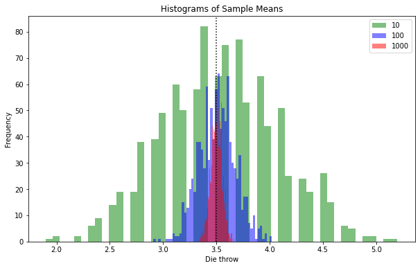
Mean of a Discrete Uniform Distribution
Now we have a statistical good picture of the mean height of our population. Now we look at the six-sided die thrown by every single inhabitant of our country. The population mean is 3.5 as every board game player should know. The shapes of the histograms of our 1,000 experiments each with the three sample sizes are again roughly normal-shaped. This is another hint at the practical usefulness of the normal distribution. Here there is obviously no direct connection between the uniform distribution of our die throws and the normal distribution of our experiments getting the statistical mean.
The discrete nature of our die throws giving us only six possible outcomes combined with the large number of bins gives us a strange looking histogram for sample size 10. The reason is that there are only a limited number of outcomes throwing a six-sided die ten times, namely all natural numbers between 10 and 60. This gives us some gaps in the histogram but still the shape resembles a normal distribution.
Again the normal distribution becomes more narrow with the number of samples and with 1,000 samples we are already really close to the population mean of 3.5 in practically all our experiments. However as the jaggedness of the curve shows there is still quite a bit of randomness involved as with the continuous normal distribution of height. This we can reduce in our setting by doing 10,000 or even 100,000 experiments with the different sample sizes. This is easily possible even with an old laptop. It is not practical in a real population as you would be better off taking a larger sample as opposed to making a lot of surveys with smaller sample sizes. If you do the math you can easily see that as opposed to asking a random sample of 1,000 people 1,000 times you can as well just do a full census and ask everybody.
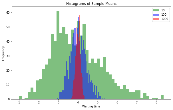
Mean of an Exponential Distribution
The pictures start repeating and we get very similar results with sampling the exponentially distributed waiting time for the next messenger message in our population. If you look closely however you will see that the small sample size of 10 tends not to be centered around the population mean of 4. The reason is that, as opposed to the uniform and the normal distribution, the exponential distribution is asymmetric. We get a few very long waiting times which distort our mean if we in one random experiment get one of them. In small samples these outliers distort the mean. In larger samples it is evened out and we look at a typical normal distribution for the means of our samples.
It is important to realize that these outliers are actually part of our data. Some people in our population were waiting e.g. 40 minutes for the next message while the average waiting time is only 4 minutes. So we are not dealing with wrong measurements. It still might be beneficial to eliminate these outliers however to get a more accurate picture of the actual mean when dealing with small samples. The issue is harder to judge when we are unaware of the distribution in your population as opposed to knowing that we are dealing with an exponential distribution.
Evaluating the Variances
For now we were looking at the population means which is typically the most relevant information. There are quite a bit more relevant statistical parameters. Maximum or minimum will not help us much in a sample except for checking for potential outliers as discussed above. Chances that we got the actual population maximum or minimum in our sample are really small. To understand the distributions in our population the variance might be helpful. Sample variance is a reasonable value to calculate.
The Mathematics
The formula for variance is:
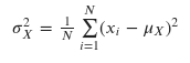
You might remember a few things about variance:
- The standard deviation is the square root of the variance. We don’t need it here but it is important to know that we are talking about the same thing basically.
- The sample variance is calculated differently. We use 1/(𝑁−1) to calculate sample variance.
It is actually even more complicated as we need to consider degrees of freedom when looking at the sample variance. In our experiments within each experiment we can use 1, so we won’t bother. The mathematical background is explained very well in this video by Michelle Lesh.
The Experiments
Looking at our experiments the summary is: You can forget about the mathematics. Dividing by 1,000 or 999 is not a big difference anyway. In theory with a sample size of 10 we should be about 10% from the population variance on average. But once we look at the distribution of our sample means and how spread out the sample variance in our 1,000 experiments with a sample size of 10 is, the conclusion is that being 10% off is not that bad at all. Most of our experiments with a sample size 10 are far more off the actual population variance.
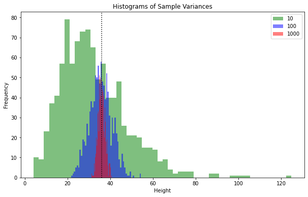
Looking at it in a Different Way
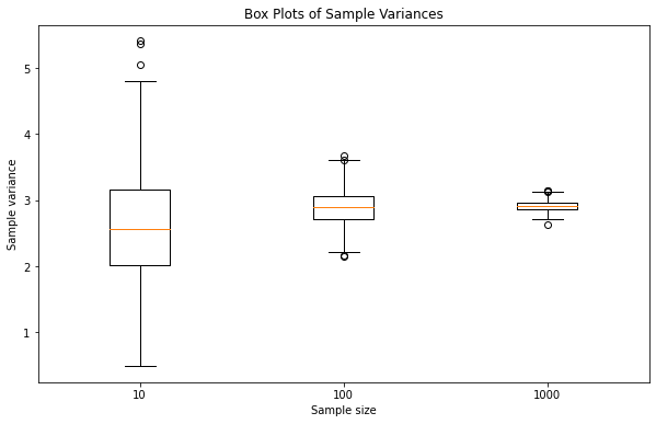
After seeing plenty of approximately normally distributed histograms we can try another visualization. The results of our experiments for variance are similar to the mean approximately normally distributed and closer to the population variance with larger sample sizes. To get a better grasp of the effect of sample size on the quality of our statistical estimate for variance we use a box plot.
The box plot gives us the mean of our 1,000 experiments plus the range of standard deviations away from our statistical mean. While everything may sound perfectly natural, looking at it in more detail is worth the effort:
- We are estimating variance using samples.
- With each sample size we make 1,000 estimates of variance.
- Over the experiments we get a mean for the statistical variance over the 1,000 estimates.
- The 1,000 experiments also have a variance which is just the standard deviation squared.
So the box plot shows us the variance of our estimates of population variance using a certain sample size. When working with experiments this comes natural. Thinking abstractly about the theory of what is happening does not make it easier.
The results look reasonable: With growing sample size we get a narrower statistical estimate of population variance. With 1,000 samples we are quite close to population variance. The box plot shows this clearer than the overlaid histograms. The information that we are dealing with approximately normally distributed random experiments is lost however. Typically it is worthwhile to try different visualizations as they tend to give different insights into the data.
fig, ax = plt.subplots(1, 1)
plt.boxplot([sample_variances[0][1], sample_variances[1][1],
             sample_variances[2][1]])
ax.set_xticklabels(['10', '100','1000'])
plt.gca().set(title='Box Plots of Sample Variances',
              xlabel='Sample size',
              ylabel='Sample variance')
plt.show()
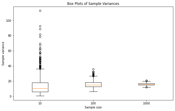
Outliers
As we already saw in the box plot of the variance for the uniform distribution, there are also outliers in our experiments. For the uniform distribution these are few and we have a roughly similar number with all sample sizes. For the very asymmetric exponential distribution this is very much different. Again as with the mean using small sample sizes we are way off.
If we get one of the more extreme values, the other samples cannot compensate for it and we get extreme results for mean or variance. This produces numerous outliers. If we have larger sample sizes we have a better chance that the other samples compensate for the extreme value when calculating mean or variance. The box plot shows this explicitly while especially outliers tend to get overlooked when working with histograms.
Conclusion
The thing to remember from this article is that it is worthwhile to do some experimenting when trying to understand complex theoretical things. And especially in probability theory and statistics this is possible with very limited effort. Python is a good tool for doing this as there are many libraries available covering even the most advanced constructs. But even Excel supports a reasonably large set of statistical functions and can be used to experiment.
Besides getting a feeling for the theory proficiency with the tool used for the experiments will also be increased. And once you have the basic elements you can easily vary your experiments. Try, for example, making 100,000 experiments as opposed to 1,000. You will still be doing random experiments but the distribution of the results will much more closely match the theoretical distributions.
Again remember that you can get the whole Python notebook on Github.
Population versus Sample was originally published in Towards Data Science on Medium, where people are continuing the conversation by highlighting and responding to this story.
from Towards Data Science - Medium https://ift.tt/Jb6I8An
via RiYo Analytics


No comments