https://ift.tt/IkXRNWY 5 minutes explanation of how anomaly detection can be improved by passing images with random patterns to the autoenc...
5 minutes explanation of how anomaly detection can be improved by passing images with random patterns to the autoencoder

In this story, I am going to review the reconstruction-by-inpainting anomaly detection (RIAD) method [1], introduced by the University of Ljubljana. There are two main concepts in this paper:
- RIAD is a method that removes partial local regions in images and reconstructs the images started by corrupted images
- RIAD is based on an encoder-decoder network, that learns to distinguish anomaly-free images from images with defects.
Outline
1. Prerequisites
Before diving into the explanation of the paper, there are some concepts that need to be known. Since the paper uses an autoencoder, you need to understand what it is. Check out my article to understand how it works.
- U-net
- How can autoencoder be applied for anomaly detection?
- Limitations of autoencoder in anomaly detection
- Reconstruction loss of autoencoder
- Structural Similarity
- Gradient Magnitude Similarity
U-net
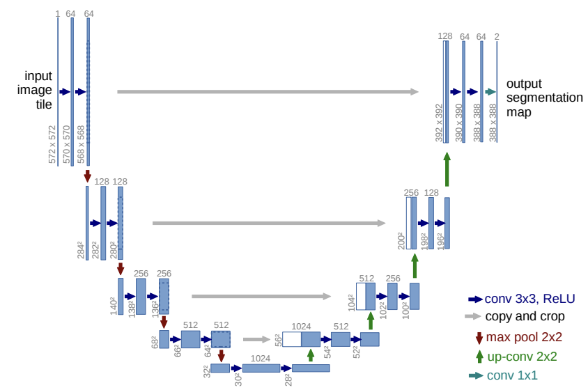
The U-net is a convolutional encoder-decoder network introduced by Ronneberger in 2015 [4]. It’s composed of two networks: the encoder to compress the patterns of the data and the decoder to decompress and rebuild the original data. The main characteristic of this network is its architecture. In the encoder architecture, the number of feature channels is doubled in each convolutional layer, while the number of channels is halved in the decoder architecture. Moreover, the U-net uses skip connections to transfer features through different layers of the network. This is an important aspect that leads to accurate reconstructions.
For better details, there is this review written by @Sik-Ho Tsang that explains the U-net’s architecture.
How can autoencoder be applied for anomaly detection?
- The detection of anomalies is a crucial challenge for a huge variety of fields, like banking, insurance and manufacturing. In this context, autoencoders can be a good fit to solve this type of problem since they can work on unsupervised problems.
- During training, you only pass normal data to the autoencoder. In this way, the model will learn the latent representation from the provided training data. We’ll also assume that the anomalous data, not observed during training, shouldn’t be reconstructed well by the autoencoder and, consequently, should have a high reconstruction error compared to normal data.
- For example, an autoencoder can be applied to solve the fraud detection problem. We pass to the model only the normal transactions during training. When we evaluate the model in the test set, most of the fraudulent transactions may have a mean squared error that is higher than the normal transactions.
Limitations of autoencoder in anomaly detection
- The autoencoder tends to learn the “identity” function
- Then, it is able to recreate the anomalous data even if it was never trained on it.
Reconstruction loss of autoencoder
The loss function to train the autoencoder is denominated reconstruction loss. The most popular reconstruction loss is the Mean Squared Error (MSE) loss function. It calculates the mean of the squared differences between the original inputs and the network outputs. If it’s applied to images, the MSE measures the average pixel-wise difference of the images we are comparing. The higher MSE is, the less similar the images are.

An alternative to the MSE is the L1 function, which measures the sum of the absolute differences between the inputs and the outputs

Although these reconstruction losses are commonly used, they have some limitations. They assume independence between neighbouring pixels, which is often not respected and, then, is not enough to measure the similarity between the original samples and the network outputs quantitatively.
Structural Similarity
To take into account local dependencies, instead of differences in single pixel values, the SSIM (Structural Similarity) loss has been proposed in many papers [2]. SSIM measures the distance between a pair of image patches p and q, which is characterized by three different aspects:
- luminance, which is taken into account through the calculation of the patches’ means.
- contrast is a function of the patch variances.
- structure is considered by calculating the covariance of two patches.

Its range of values is between -1 and 1. When the score is near 1, it means that the two compared images are similar, whereas the score of -1 indicates that they are very different.
Gradient Magnitude Similarity
Like SSIM, Gradient Magnitude Similarity is a measure of the local similarities between the compared images [3]. Instead of comparing image pixels, it takes into account the local gradients across two images I and I_{R}.

where g(I) is the gradient magnitude map for the image I and c is a constant to ensure numerical stability.

2. MVTEc AD dataset
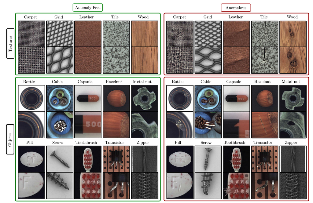
The MVTec AD is a novel and comprehensive industrial dataset
consisting of 5354 high-resolution images with 15 categories: 5 types of tex-
tures and 10 types of objects [5]. The training set is composed of only normal
images, while the test set contains both defect and defect-free images. The
image resolutions are variable between 700x700 and 1024x1024 pixels
3. RIAD algorithms
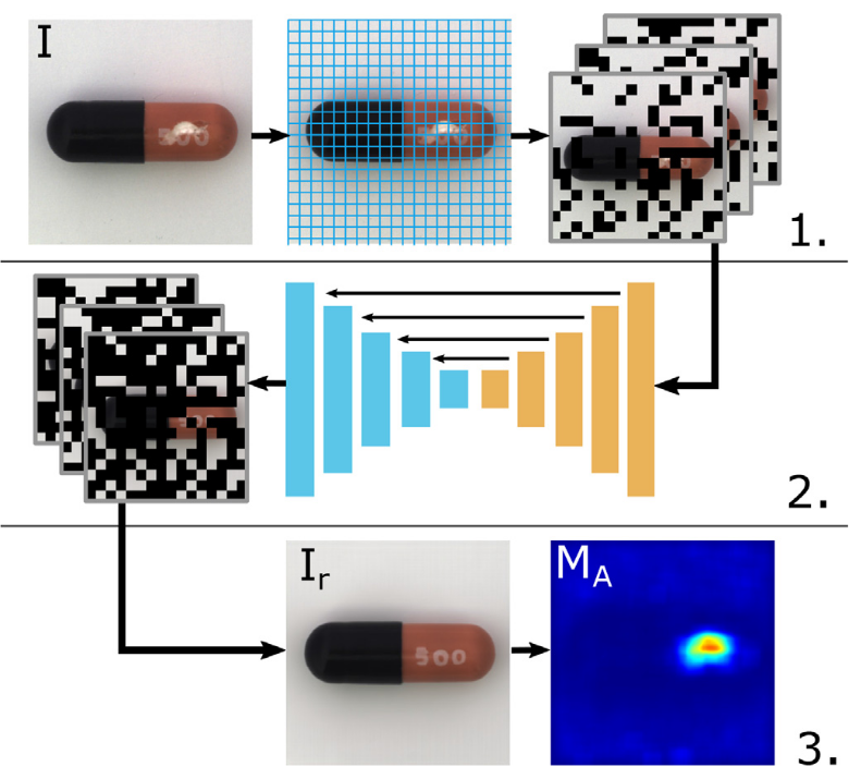
The autoencoder is trained on anomaly-free images, from which randomly selected regions are set to 0. The encoder-decoder architecture used is the U-net, as explained previously. But how are these images masked? These are the following steps:
- We select randomly a set of pixels from each image by giving in input the region size parameter k.
- Each image can be considered as a grid of dimensions Height/k * Width/k.
- Our image/grid is randomly split up into n disjoint (or non-overlapping) sets Si.
- We generate a binary mask, M_{Si}, that contains 0 if the local regions belong to the set Si, and 1 otherwise.
- The final image is the product between the binary mask and the original image.
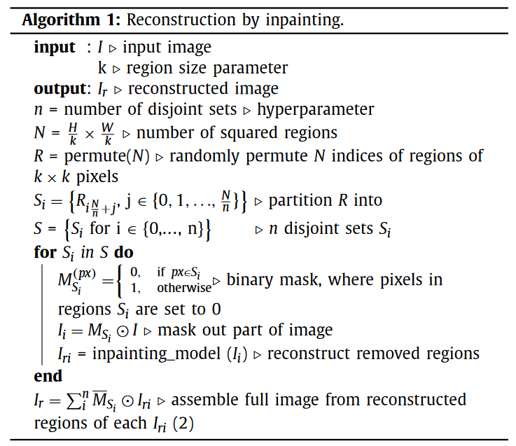
During the training of the U-net, the size k is selected randomly from a set of values K. In the paper, they use K = {2,4,8,18} as a set of region sizes. After the mask is applied to the original images, the reconstructions are obtained by giving the inpainted images to the model and, then the total loss is calculated by taking into account three types of loss:
- MSGMS loss, which is the average GMS distance at several scales:

where Hl and Wl are respectively the height and the width of the images compared, Nl is the number of pixels at scale l.
- SSIM loss is the average of all the local SSIM values:

- pixel-wise L2 loss (or the mean squared error loss)
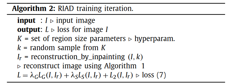
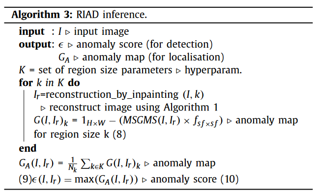
During the evaluation of the model, each test image is inpainted for each value of k. Then, we can obtain the average of the anomaly maps G_A(I, I_{R}) produced for each image reconstruction I_{R} at each value of k. Later, we compute the image level anomaly score, which is essentially the maximum of the average of the anomaly maps.
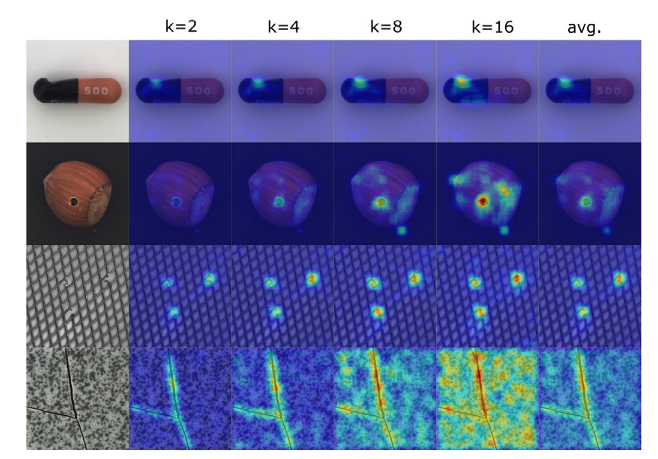
For example, let’s suppose that K = {2,4,8,16}. We compute the anomaly map for each image reconstruction at each value of k belonging to {2,4,8,16} and, then, we calculate the average of these anomaly maps, which is shown in the last column.
4. Results
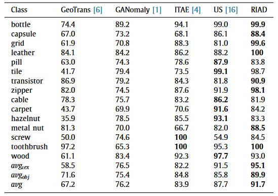
- In comparison with the other state-of-art models, RIAD outperforms on object classes, like bottle, metal_nut and toothbrush, that present high average ROC-AUC, and also achieve good results with some texture categories, such as grid and leather.
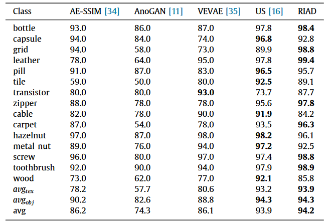
- This table shows the results for anomaly localization on the classes of MVTec AD dataset.
- It achieves higher overall ROC-AUC scores for anomaly localization compared to the other state-of-art methods.
References
[1] Reconstruction by inpainting for visual anomaly detection, Vitjan Zavrtanik, Matej Kristan, Danijel Skocaj, (2021)
[2] Improving Unsupervised Defect Segmentation by Applying Structural Similarity to Autoencoders, Paul Bergmann, Sindy Lowe, Michael Fauser, David Sattlegger, Carsten Steger
[3] Image Quality Assessment Techniques Show Improved Training and Evaluation of Autoencoder Generative Adversarial Networks, Michael O. Vertolli, Jim Davies, Carleton University, (2017)
[4] U-Net: Convolutional Networks for Biomedical Image Segmentation, Olaf Ronneberger, Philipp Fischer, Thomas Brox, (2015)
[5] The MVTec Anomaly Detection Dataset: A Comprehensive Real-World Dataset for Unsupervised Anomaly Detection, Paul Bergmann, Kilian Batzner, Michael Fauser, (2021)
Github Repository
Paper Review: Reconstruction by inpainting for visual anomaly detection was originally published in Towards Data Science on Medium, where people are continuing the conversation by highlighting and responding to this story.
from Towards Data Science - Medium https://ift.tt/WTRsnj4
via RiYo Analytics

ليست هناك تعليقات