Geospatial Site-Selection Analysis Using Cosine Similarity

https://ift.tt/AXF2gkf Identifying similarities between geographic areas based on neighbourhood amenities Photo by Wyron A on  Unsplash ...

https://ift.tt/AXF2gkf

Identifying similarities between geographic areas based on neighbourhood amenities

Photo by Wyron A on Unsplash

Introduction

Location is paramount for businesses that operate physical locations, where it is key to be located close to your target market.

This challenge is often the case for franchises that are expanding into new areas where it is important to understand the ‘fit’ of a business in a new area. The aim of this article is to explore this idea in more detail, to evaluate the suitability of a new location for a franchise based on the characteristics of areas where existing franchises are located.

To achieve this we will be taking data from OpenStreetMap of a popular coffee shop franchise in Seattle, to use information about the surrounding neighbourhood to identify new prospective locations that are similar.

Framing the problem

To approach this task there are a few steps that need to be considered:

1. Finding existing franchise locations
2. Identifying nearby amenities around these locations (which we will assume gives us an idea about the neighbourhood)
3. Finding new potential locations and their nearby amenities (repeating steps 1 & 2)
4. Evaluating the similarity between potential and existing locations

As this task is geospatial, using OpenStreetMap and packages like OSMNX and Geopandas will be useful.

Collecting the data

Finding existing franchise locations

As mentioned, we will use a popular coffee shop franchise to define the existing locations of interest. Collecting this information is rather straightforward using OSMNX, where we can define the geographic place of interest. I have set the place of interest as Seattle (USA), and defined the name of the franchise using the name/brand tag in OpenStreetMap.

import osmnx
place = 'Seattle, USA'
gdf = osmnx.geocode_to_gdf(place)

#Getting the bounding box of the gdf
bounding = gdf.bounds
north, south, east, west = bounding.iloc[0,3], bounding.iloc[0,1], bounding.iloc[0,2], bounding.iloc[0,0]
location = gdf.geometry.unary_union

#Finding the points within the area polygon
point = osmnx.geometries_from_bbox(north, south, east, west, tags={brand_name : 'coffee shop'})
point.set_crs(crs=4326)
point = point[point.geometry.within(location)]

#Making sure we are dealing with points
point['geometry'] = point['geometry'].apply(lambda x : x.centroid if type(x) == Polygon else x)
point = point[point.geom_type != 'MultiPolygon']
point = point[point.geom_type != 'Polygon']

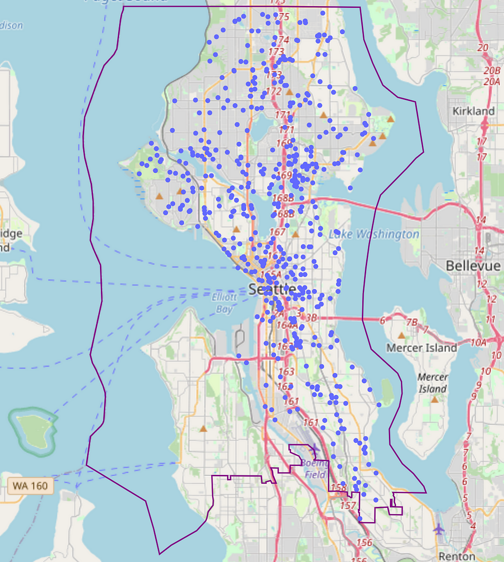
This gives us the locations of existing franchise locations with our area:

Map of existing franchise locations (blue points) within the defined Seattle area (purple polygon). Image by Author.

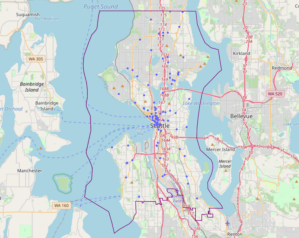
Looking at the existing locations makes us wonder about the following:

1. What is the density of the franchise in this areas?
2. What is the spatial distribution of these locations (clustered close together or evenly spread out)?

To answer these questions we can calculate the franchise density using the defined area polygon and the count of existing franchises, which gives us 0.262 per SqKm. Note: large areas in the polygon are water, therefore the density will appear much lower here than in reality…

For measuring how dispersed these locations are relative to each other we can calculate the distance to the nearest neighbour using Sklearn’s BallTree:

Map of existing franchise locations, coloured by distance to nearest neighbour (in Km), within the defined Seattle area (purple polygon). Image by Author.

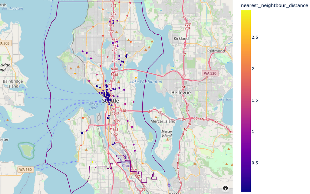
Nearest neighbours can also be shown as a histogram:

Nearest neighbour histogram. Image by Author.

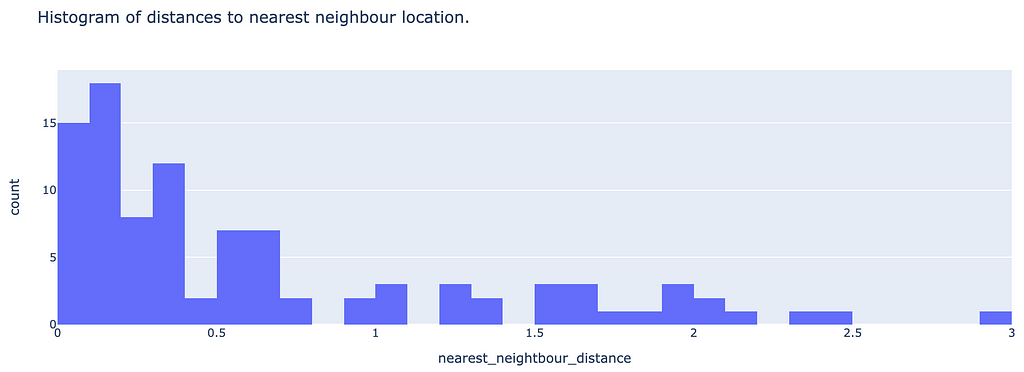
It looks like the majority of locations exist with 800m of each other, which is apparent when looking at the map and seeing the high density of existing locations in the city centre.

What about the amenities surrounding these locations?

We first need to get all the amenities within an area of interest and define a radius around each existing location, that can be used to identify nearby amenities. This can be achieved using another BallTree, however querying points based on a specified radius (which I’ve set as 250m):

from sklearn.neighbors import BallTree

#Defining the tree based on lat/lon values converted to radians
ball = BallTree(amenities_points[["lat_rad", "lon_rad"]].values, metric='haversine')

#Querying the tree of amenities using a radius around existing locations
radius = k / 6371000
indices = ball.query_radius(target_points[["lat_rad", "lon_rad"]], r = radius)
indices = pd.DataFrame(indices, columns={'indices'})

When we query OSM and use the BallTree to find nearby amenities we are left with the indices of each amenity within the radius of an existing franchise location. Therefore we need to extract the amenity type (e.g., restaurant) and count each occurrence to get a processed dataframe like the following:

Example dataframe summarising amenities within a radius around existing locations. Each row represents an existing franchise location. Image by Author.

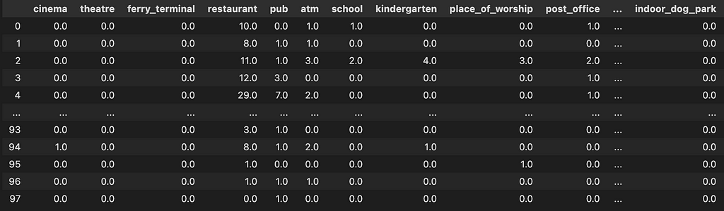
Now we can see the most popular amenities located near existing franchise locations in a sorted bar chart:

Bar chart of amenities within the radii of existing franchise locations. Image by Author.

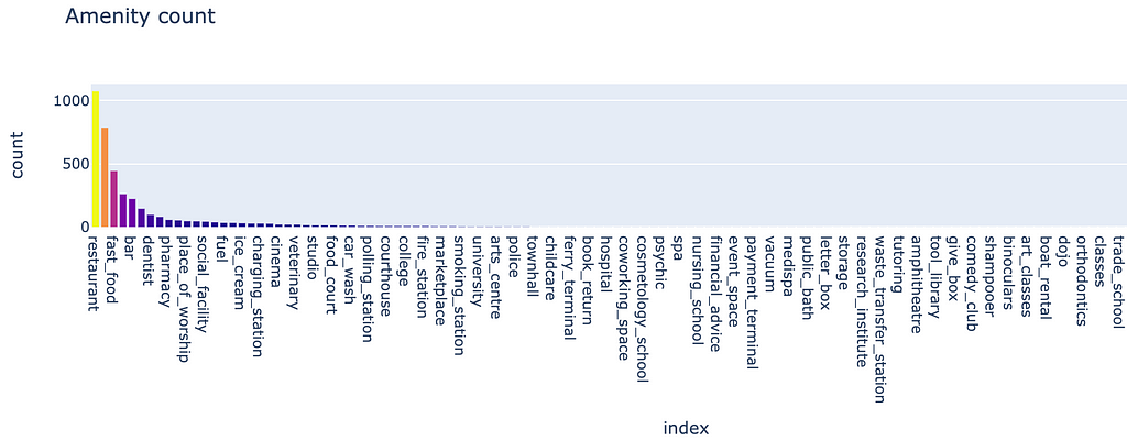
It appears that our coffee shop franchise is dominantly located proximal to other locations that serve food/drinks, along with a few other minority amenities like ‘charging station’. This gives us the total count for all existing locations, but are the distribution of amenities the same?

We can apply quick PCA and DBSCAN clustering to see how existing franchise locations cluster relative to each other (using a min_sample value of 3):

DBSCAN clustered franchise locations, coloured by cluster label. Image by Author.

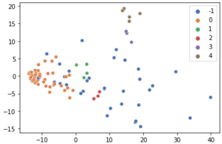
There is a dominant cluster towards the left, however other smaller clusters exist too. This is important as it tells us that existing franchise locations vary based on their surrounding amenities and do not conform to a single ‘type’ of neighbourhood.

Finding new locations

Now that we have created a dataset for existing franchise locations, we can now produce a similar dataset for new potential locations. We can randomly select nodes that exist in our area of interest using the graph extracted by OSMNX, as points will be constrained to existing paths accessible for walking:

G = osmnx.graph_from_place(place, network_type='walk', simplify=True)
nodes = pd.DataFrame(osmnx.graph_to_gdfs(G, edges=False)).sample(n = 500, replace = False)

Randomly sampled locations (blue) that we will compare against the existing franchise locations. Image by Author.

Finding nearby amenities for each of these potential locations can be achieved by repeating the previous steps…

A slightly messy location map highlighting existing franchises (black), new prospective locations (dark green), and all amenities in the area (coloured by amenity type).

Measuring the similarity between existing and potential locations

This is the part we’ve been waiting for; measuring the similarity between existing and our potential locations. We will use the pairwise cosine similarity to achieve this, where each location consists of a vector based on the diversity and quantity of amenities nearby. Using cosine similarity offers two benefits in this geospatial context:

1. Vector lengths do not need to match = We can still measure similarities between locations with different types of amenities.
2. Similarity is not based on just the frequency of amenities = Since we also care about the diversity of amenities, not just the magnitude.

We calculate the cosine similarity of a potential new location against all other existing locations, which means that we have multiple similarity score.

max_similarities = []
for j in range(len(new_locations)):
similarity = []
for i in range(len(existing_locations)):
cos_similarity = cosine_similarity(new_locations.iloc[[j]].values, existing_locations.iloc[[i]].values).tolist()
similarity.extend(cos_similarity)
similarity = [np.max(list(chain(*similarity)))]
average_similarities.extend(similarity)
node_amenities['averaged similarity score'] = max_similarities

So how do we define what is similar?

For this, we can remember that existing locations do not form a single cluster, meaning there is heterogeneity. A good analogy can be when evaluating a person can join a friendship group:

1. A friendship group typically will contain different people with varying traits, and not a group of people with identical traits.
2. Within a group, people will share more or less traits with different members of the group.
3. A new potential member doesn't necessarily need to be similar to everyone in the group to be considered a good fit.

Because of this, we chose the maximum similarity score when comparing with existing locations, as this tells us that the potential location is similar to at least one other existing franchise location. Taking an average would lead to lower score, since variation in nearby amenities exists between franchise locations. We can now plot the results, coloured by similarity score, to see what areas could be new franchise locations:

Potential locations coloured by similarity score (where yellow represents high % similarity and purple means no similarity), alongside existing franchise locations (black). Image by Author.

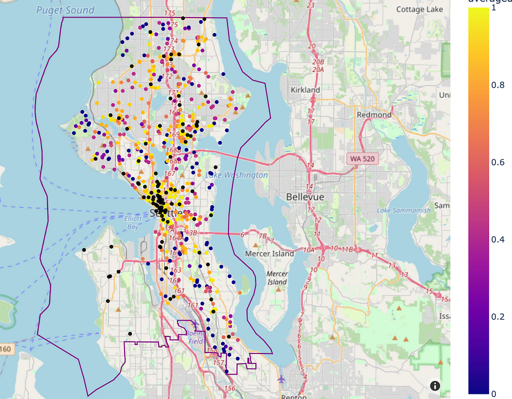
Our similarity scores for locations in the city centre all show strong similarities with existing locations, which makes sense, therefore what we’re really interest in are the locations with high similarity scores that are positioned far away from existing franchise locations (black points on the map).

Final thoughts

We have used geospatial techniques to evaluate the potential locations for a coffee shop franchise to expand into new locations, using cosine similarity scores based on nearby amenities. This is just a small piece of a bigger picture, where factors such as population density, accessibility etc. should also be taken into account.

Keep an eye out for the next article where will start to mature this idea further with some modelling. Thanks for reading!

---

Geospatial Site-Selection Analysis Using Cosine Similarity was originally published in Towards Data Science on Medium, where people are continuing the conversation by highlighting and responding to this story.

from Towards Data Science - Medium https://ift.tt/QsgPzCE
via RiYo Analytics