https://ift.tt/1XDh5Ym How well does Deep Gaussian process modeling quantify the uncertainty in your signal Image by the author Advance...
How well does Deep Gaussian process modeling quantify the uncertainty in your signal

Advanced machine learning (ML) techniques nowadays can answer pretty sophisticated questions derived from your data. Unfortunately, due to the “black-boxiness” of their nature, it is difficult to assess how correct those answers are. It might be fine if you are trying to find pictures of cats in your family album. But in my line of work, processing medical data, it is borderline unacceptable, thus oftentimes preventing the practical use of ML models for real clinical applications. In this post I would like to outline an approach to the analysis of biological data that combines both, the complexity of the modern ML and the reasonable confidence assessment of classical statistical methods.
What are we talking about here?
My goal is to provide
- the rational for using Gaussian process modeling for biological data and, specifically, deep Gaussian process (DGP) rather than an ordinary, stationary one
- an overview of Hamiltonian Monte Carlo (HMC) method and how it helps with DGP modeling
- an illustration of application of this approach on an example of simulated data
Challenges of analyzing medical data
Imagine that we are a group of doctors and we are monitoring a patient who has been treated for something. Let’s say that treatment is supposed to affect levels of a certain hormone. We are recording the test results over time and gradually getting a picture like this.
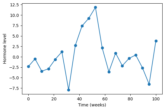
This is obviously a very noisy data. We cannot immediately tell what is going on, but we really want to know if the hormone levels are changing. Usually, the first thing people do, to see if there is any effect, is the good old linear regression that lumps all noise into a random normal. In the majority of real world clinical data this gives little. So, the second best thing to do is to model this as a Gaussian Process (GP). Why does it make sense? Well, first of all, let us review what a GP is.
Viewing clinical signals as a Stationary Gaussian Process
When a GP modeling is performed, all the data points are considered to be drawn from multivariate Gaussian distribution as
Two points to note. 1) K(X) here is a square matrix the size of your data and, in a general case, has non-zero off-diagonal elements; that makes it different from considering your data as n independent random draws. 2) The data points are indexed by X, like, in our example, time, defining the order — thus, the process. That is pretty much all we need to know about GPs for the purposes of this post. However, this topic is well studied, and a curious reader can find an excellent source for extending their knowledge in the classic reference [1].
When we talk about fitting a GP, we mean finding the parameters of the matrix K(X). To make it more explicit, let us re-write a GP model as
Now we have three parameters, and I would like to make an argument, that they can be interpreted as capturing different aspects of the process that we are trying to model here. Here is the argument.
When a time-varying medical signal is analyzed, we are trying to assess an evolution of some biological process through medical tests. That evolution happens on the background of a lot of noise. Come to think of it, we can separate the sources of noise in roughly two categories. One is the measurement noise and, as the tests get pretty sophisticated in modern medicine, this component might have a fairly complex structure. The other source is the variation caused by biological processes in a living being NOT related to the process that we are interested in. That part is even more complicated and substantially less studied. Than, the actual signal, representing the process that we are trying to detect, might be highly nonlinear. All of that creates a big mess of a data and we have no chance to model it precisely, at least not in foreseeable future.
But we can make an attempt to model these three components semi-separately in the framework of a GP. Most likely, the two sources of the noise have different frequency and amplitude. First of all, the g parameter is a descendant of the random noise in linear regression analysis. Technically, it would be τ²g, but that where the “semi-separately” comes from, and it is also easily accountable for. It would be most natural to connect this parameter to the measurement noise. This type of noise does not change from patient to patient as long as we are talking about the same type of measurement. It even might be per-trained from repeated tests and kept fixed. The biological noise we assign to be represented by τ². The reason for that is, that this parameter is responsible for the amplitude of the variation. This is most likely patient-dependent, but remains more or less constant during the monitoring time of the same patient. Than, there remains θ which is responsible for describing how closely the data points are correlated between each other. If we are observing a patient under treatment, and the treatment is actually taking an effect, then it would be reflected in the consecutive measurements to be strongly correlated. So, the θ parameter is reserved for the signal that we are trying to detect.
As we can see, a GP model can neatly accommodate our needs for putting some math behind medical data. It is a nice step up from linear regression. But there is one problem. All the parameters of the model are assumed to remain constant. That could be fine for g and τ² parameters because, as we argued above, they are attributed to the measurement noise and the biological variations in the body not affected by the treatment. But we cannot count on the same for θ. The treatment can be stopped, or changed, or it could stop working on its own. That would affect the correlation in the signal and we would like to know that. Therefore, we have to allow for θ to change.
The solution comes with a Deep Gaussian Process model. Just like with the deep neural networks, it implies adding more layers.
Two-layer GP as a more adequate alternative
There are many ways to add layers to a GP. For our purpose, we simply insert another GP between the time indices and the measured signal like this
following the methodology of reference [2]. Why is that enough? As we mentioned above, we only need to accommodate changing θ. By introducing an additional GP for the time variable, we are “warping” the spacing between the measurement time points in a flexible manner and that produces the desired effect.
But it also complicates the fitting! Somehow we have to find optimal values of the parameters for our data from this posterior distribution

with the two likelihoods defined as
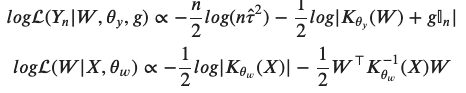
For the derivation of this expression see reference [2]. Now that we wrote out this monstrosity, we need to think how make something useful out of it. Not much can be done analytically here. The most straightforward way is to sample this distribution numerically. And the best way to sample numerically is the Hamiltonian Monte Carlo!
A taste of Hamiltonian Monte Carlo method
We need a smart approach to sample our distribution for two reasons, that are actually two views of the same thing. The thing is that we have our probability distribution defined in a multidimensional space. The space is big, but the probability has to be finite. This means that non-zero regions of probability will be confined to small volumes in space. But those are the volumes where we want to be. So the two reasons that we cannot just blindly throw the darts are 1) waste of time — we will spend a lot of time in regions with zero probability and it will be useless; 2) inaccurate estimates — at some point we would have to stop sampling, and there is a chance that we will miss non-zero regions.
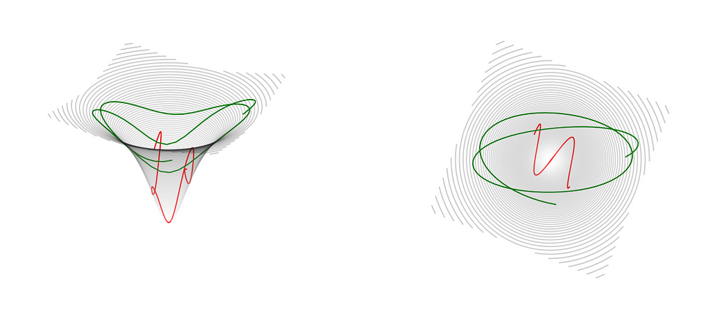
The solution comes from drawing the analogy to a particle motion as described by a well-known mechanism in physics. Imagine a charged particle flying through space near an opposite charge, or an actual physical hard cone turned upside down and you are sliding a ball down the side. In all these cases, the moving object is attracted and moves towards the bottom part of the cone or the place where the oppositely charged particle is located. But if it has enough speed to begin with, if you push the ball hard enough sideways, it will bounce around this center of attraction. This figure shows just that — two possible trajectories with different initial velocities, or momentum, how we say in physics. The green one has a higher momentum than the red, so it spends a little more time farther away from the center. But both of them are going towards it.
This situation is described in theoretical mechanics by Hamiltonian equations
where
is the sum of kinetic and potential energies. As a physicist I cannot stop admiring the simplicity and beauty of these equations.
Making HMC work for us
All we have to do now is to say that our probability distribution is the U, the potential energy. To turn it upside down, we put a minus sign in front of it, as it is already written in our equation, and start solving Hamilton equations with different values of momentum to explore regions around the maximum. A lot of details of HMC can be found in reference [3]. Here is an example code that I have written to generate one such trajectory.
As we might notice, there is a little hiccup — we need a derivative of our probability function, grad_U, to be supplied.
It is not possible to come up with an analytical expression for the derivative of the log likelihood with respect to any of the parameters. Of course, we can try a numerical method of estimating the gradient, but I decided to test out the tensorflow library, which, I suppose, is still numerical in the end, but a little more elegant. Below is a snippet of my code that implements the log likelihood using tensorflow functions (the whole code is too big and boring). For the derivative it uses the GradientTape. It actually works wonders!
How did it work?
I have to confess, that the hypothetical plot of the patient data in the beginning of my post was totally fake. It was simulated the following way.
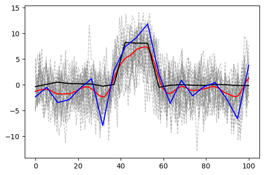
That is, it is drawn from a multivariate Gaussian with dimension 20, having mean zero everywhere except in the middle three positions where it is 4, and the covariance matrix with first off-diagonal elements all 0.1. I multiplied the whole thing by 2 just for kicks. I generated 60 samples. I picked one out and added random normal noise to it with variance 1. This is shown in the figure below — the blue line is the sample that I picked, the blue dots are that sample with the added noise, grey dashed lines are the remaining samples drawn from the same distribution, and the black line is their mean.
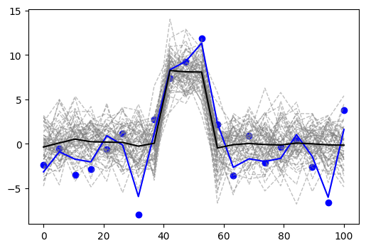
The grey lines in the background are meant to give us a visual estimate of uncertainty in the data that comes from this distribution. The reason why it is useful is that, as an additional bonus of our approach, we will try to estimate that uncertainty based on one sample that we are given. Of course, the main goal is to estimate the black line — the signal.
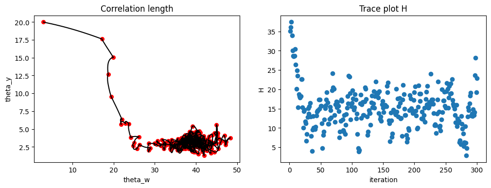
I fed the one sample with noise, the blue dots from the picture above, to my implementation of two-layer GP with HMC. Here are the results. First of all, let us look at the conversion. We have 24 parameters here (τ²,g,θ_y,θ_y, and 20 Ws), so it is not possible to show the full space. The picture below shows just two of the parameters, the two θs on the left. I deliberately started far from the correct values, but notice how quickly the trajectory moves towards a stationary point, presumably the maximum of the probability, and starts hovering around it. The plot on the right shows the total energy vs the number of iterations. Again, quick move to, hopefully, minimum and good mixing around it.
Here is the inferred signal. I inferred 200 samples using the sampled posterior values for the parameters, appropriately discarding the initial burn-in samples. The result is shown in the picture below, where the blue and the black lines represent the original sample and the mean of the real data, respectively. The red line is the mean of the inferred samples. The gray dashed lines are all the individual inferred samples to be compared with the figure above for the simulated data.
In the end, this is what our net result would be. The black — the signal we are trying to recover, the red — our best guess at it, and the dashed grey — 95% confidence intervals around our guess.
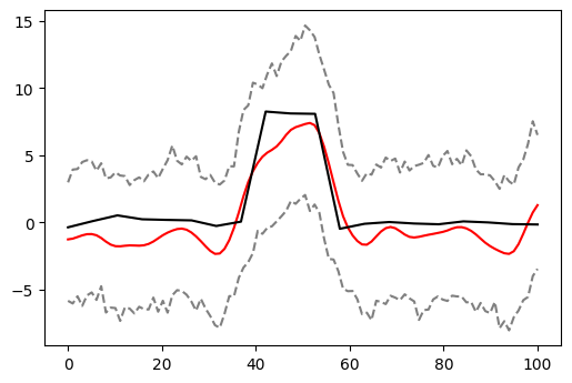
Yes, those confidence intervals might be a tad wider than the real thing, but we would have a definite detection of the change in the signal in the middle and we would not be fooled by the wiggling on the sides. Considering how little we were given (one sample with various sources of variation and no replicates), this is a pretty powerful result, don’t you think?
References
[1] C. E. Rasmussen and C. K. I. Williams, Gaussian Processes for Machine Learning, (2006), The MIT Press ISBN 0–262–18253-X.
[2] A. Sauer, R. B. Gramacy, and D. Higdon, (2021) Active Learning for Deep Gaussian Process Surrogates, arXiv:2012.08015v2
[3] M. Betancourt, A Conceptual Introduction to Hamiltonian Monte Carlo, (2018), arXiv:1701.02434
Thank you for reading. I would be happy to answer any questions and hear any comments. I extend the special thanks to Robert Gramacy and Annie Sauer for stimulating discussions, and to the reviewers from Towards Data Science.
Fitting Deep Gaussian Process via Hamiltonian Monte Carlo was originally published in Towards Data Science on Medium, where people are continuing the conversation by highlighting and responding to this story.
from Towards Data Science - Medium https://ift.tt/2xftn8Z
via RiYo Analytics


ليست هناك تعليقات