https://ift.tt/OrQpZxc A step-by-step guide to implementing k-means clustering for customer segmentation with Python Photo by Isaac Smith...
A step-by-step guide to implementing k-means clustering for customer segmentation with Python

In my previous article, we started our journey to implement the popular STP marketing framework, in this post, we’ll continue the voyage by overcoming the limitations of hierarchical segmentation with one of the most popular unsupervised machine learning algorithms “k-means clustering”.
As before the entire notebook and reference data are available in the Deepnote notebook.
Table of contents
  ∘ Introduction
  ∘ Implementing K-Means Clustering
  ∘ Observations
  ∘ Visualize our customer segments
  ∘ Conclusion
Introduction
Hierarchical clustering is great for small datasets, but as the dataset size grows, the computational demands grows rapidly. Because of this, hierarchical clustering isn’t practical, and in the industry flat clustering is more popular than hierarchical clustering. In this post, we are going to use the k-means clustering algorithm to divide our dataset.
There are many unsupervised clustering algorithms out there, but k-means is the simplest to understand. K-means clustering can segment an unlabeled dataset into a pre-determined number of groups. The input parameter ‘k’ stands for the number of clusters or groups we would like to form in the given dataset. However, we have to be careful in choosing the value for ‘k’. If the ‘k’ is too small, then the centroids won’t lie inside the clusters. On the other hand, if we choose ‘k’ as too big, then some of the clusters may be over-split.
I’d recommend the following post to learn more about the k-means clustering:
Understanding K-means Clustering in Machine Learning
Implementing K-Means Clustering
The way the k-means algorithm works:
- We choose the number of clusters ‘k’ we’d like to have
- Randomly assign the cluster centroids
- Until clusters stop changing, repeat the following:
i. Assign each observations to a cluster for which the centroid is the closest
ii. Compute the new centroid by taking the mean vector of points in each cluster
The limitation of the k-means algorithm is that you have to decide beforehand how many clusters you expect to create. This requires some domain knowledge. In case, you don’t have the domain knowledge, you can apply the ‘elbow method’ to identify the value of ‘k’ (number of clusters).
This method essentially is a brute-force approach, where you calculate the sum of the squared distance between each member of the cluster and its centroid for some value of ‘k’ (e.g. 2–10) and plot ‘k’ against the squared distance. As the number of clusters increases, the average distortion will decrease, meaning the cluster centroids move closer to each data point. In the plot, this will produce an elbow-like structure hence the name ‘elbow method’. We’ll choose the value of ‘k’ at which the distance decreases abruptly.
As we can see in the above graph, the line declines stiffly until we reach the number of cluster 4, and declines more smoothly after that. Meaning that our elbow is at 4 and that is the optimal number of clusters for us. This also aligns with the output of hierarchical clustering that we did in the previous article.
Now let’s perform k-means clustering with 4 clusters, and include the segment number with our dataframe.
Observations
Great, we’ve segmented our customers into 4 groups. Now let’s try to understand the characteristics of each group. At first, let's see the mean value of each feature by clusters:
Here are some of my observations:
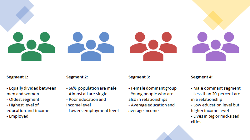
From the above observations, it feels to me that segments 1 and 4 are well-off with higher income and better occupations compared to segments 2 and 3.
It’s always better to assign appropriate names to each group.
1: 'well-off'
2: 'fewer-opportunities'
3: 'standard'
4: 'career-focused'
Let’s take a look at the number of customers per segment:
Visualize our customer segments
Age vs Income:
Education vs Income:
Conclusion
We observe in the ‘age vs income’ scatter plot that higher age customers with higher income (well-off) are separated, but the other three segments are not that distinguishable.
In the second observation, ‘education vs income’ violin plot, we see that customers with no educational records have lower income, and those who graduated have higher income. But other segments are not that separable.
Following these observations, we can conclude that k-means did a decent job separating the data into clusters. However, the outcome is not that satisfactory. In the next post, we’ll combine k-means with principal component analysis and see how we can achieve a better result.
Customer Segmentation with Python (Implementing STP Framework—Part 2) was originally published in Towards Data Science on Medium, where people are continuing the conversation by highlighting and responding to this story.
from Towards Data Science - Medium https://ift.tt/4hDg9m3
via RiYo Analytics


No comments