https://ift.tt/fNnUBdQ A step-by-step guide to implementing hierarchical clustering for customer segmentation with Python Photo by Isaac ...
A step-by-step guide to implementing hierarchical clustering for customer segmentation with Python

I’m starting a new blog post series, where I’ll show you how to apply the popular STP marketing framework step by step with Python. STP (Segmentation, Targeting, Positioning) is a well-known strategic approach in modern marketing which helps you to understand your customer groups (segments) and place your products to the targeted audience more effectively. This is an approach that transitions from a product-centric approach to a customer-centric approach. STP framework allows brands to develop more effective marketing strategies, hyper-focused on the targeted audience’s wants and needs.
In this blog post series, I’ll describe how to know your customers better through segmentation and we’ll see different approaches there, then we’ll see how to position yourself so that you serve your customers better.
This first post is going to focus on understanding and preprocessing the dataset, and segmenting our customers in a simplistic way.
In the upcoming post, we’ll apply a more sophisticated way of segmentation.
The entire notebook and reference data are available in the Deepnote notebook.
Table of contents
  ∘ STP Framework
  ∘ Environment Setup
  ∘ Data Exploration
  ∘ Data Preprocessing
  ∘ Hierarchical Clustering
  ∘ Conclusion
STP (Segmentation, Targeting, Positioning) Framework
Segmentation helps you divide your potential or existing customers into different groups depending on their Demographic, Geographic, Psychographic, and Behavioral characteristics. Customers of each group share similar purchase behaviors and are likely to act similarly in different marketing activities. A generic marketing campaign like “one size fits all” doesn’t work best as a marketing strategy.
Targeting: Once you know your customer segments, the next step is to select a subset of segments to focus on. It’s hard to make a product that satisfies everybody. That’s why it’s best to concentrate on the most important group of customers and make them happy. Later you can always increase your focus area and target more customers.
The most important considering factors while choosing your target segments are:
- Size of the segment(s)
- Growth potential
- Competitor’s target segment & offerings
Targeting activities utilize qualitative examinations and fall into the advertising domain. That’s why we will not focus on the targeting phase in this blog series.
Positioning: In this step, you map out the different attributes considered in the previous two steps and then position your product. This helps you identify what products and offerings you want to offer that will best satisfy your customer’s needs. The positioning also guides you on how those products should be presented to the customers and through what channel. There is another framework used in this process, called Marketing Mix. I’ll describe Marketing Mix briefly when we reach that module.
Environment Setup
In this entire series of tutorials, I’m going to use Deepnote as the only development tool. Deepnote is an awesome Jupiter-like web-based notebook environment, which supports a multi-user development eco-system. Deepnote by default comes with the latest Python and prominent data-science libraries installed. It’s also very easy to install other libraries if needed through ‘requirements.txt’ or regular bash command.
In the future, I’ll write a separate post on how to use Deepnote more effectively.
Data Exploration: Get to know the dataset
We are going to use a pre-processed FMCG (Fast Moving Consumer Goods) dataset, which contains customer details of 2000 individuals as well as their purchase activities.
It’s a good practice to look at the dataset with Excel because scrolling and skimming through the dataset is easier in Excel (as long as the dataset is not super big). Thankfully Deepnote offers an even better browsing experience for CSV datasets. It shows a distribution chart per column, which gives you an idea of each variable at a glance.
Let’s load the customer dataset into the notebook using the Pandas library.
We can see that we have an ID column and seven other demographic and geographic variables for each customer.
Here is a short description of each variable:
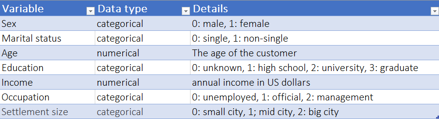
After loading the dataset into a pandas data frame, we can apply the ‘describe’ method to have a summary of the dataset. This shows some descriptive statistics of our dataset.
For numeric variables, the output includes count, mean, std, min, max as well as 25, 50, and 75 percentiles. For categorical variables, the output will include count, unique, top, and frequency.
Let’s move on with our data exploration and have a look at the pairwise correlation of variables. Correlation describes the linear dependency between variables and it ranges from -1 to +1. Where +1 indicates a very strong positive correlation and -1 indicates a strong negative correlation. A correlation of 0 means these two variables are not linearly dependent.
The diagonal values in the correlation matrix are always one because it represents the correlation of a variable with itself.
Unfortunately, it’s hard to get a general understanding of the relationships between the variables by simply looking at numbers. So let’s plot these numbers in a heat map with Seaborn.
With this heat map, we see that there is a strong positive correlation between age and education or between occupation and income. These inter-variable correlations will be important in the feature selection of the segmentation process.
To understand the pairwise relationship between variables we can use a scatter plot. In the Deepnote notebook, you’ll find examples of scatter plots.
Data Preprocessing
Even though the customer data that we are working with is clean, we haven’t performed any statistical processing of the data.
Most machine learning algorithms use Euclidean distance between two data points when calculating the distance between individual records.
When the scale of features differs in our dataset, this calculation doesn’t perform well. For example, even though 5kg and 5000gms mean the same thing, an algorithm will weigh heavily on the high magnitude feature (5000gms) in the distance calculation.
That’s why, before feeding data into any machine learning or statistical model we must standardize the data first and bring all features to the same level of magnitudes.
Why, How and When to Scale your Features
Scikit-learn offers this handy class “StandardScaler” under preprocessing module, which makes it super easy to standardize our data frame.
Hierarchical Clustering
We’ll use the dendrogram and linkage from Scipy’s hierarchy module for clustering the dataset.
A dendrogram is a tree-like hierarchical representation of data points. It is most commonly used to represent hierarchical clustering. Linkage, on the other hand, is the function that helps us to implement the clustering. Here we need to specify the method to compute the distance between two clusters, and at completion, the linkage function returns the hierarchical cluster in a linkage matrix.
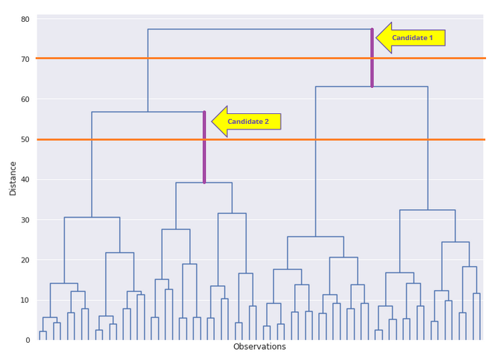
At the bottom of the plot on the x-axis, we have the observations. These are the 2000 individual customer data points. On the y-axis, we see the distance between points or clusters represented by the vertical lines. The smaller the distance between points, the further down in the tree they’ll be grouped together.
Identify the number of clusters manually
It’s great that the linkage object can figure out the optimal number of clusters for us, and the dendrogram can represent those clusters with different colors. But what if we had to identify those clusters from the dendrogram? The process is to slice through the biggest vertical line that is not intercepted by any extended horizontal line. And after the slice, the number of clusters under the slicing line would be the best number of clusters.
In the following diagram, we see two candidate vertical lines, and between them, “candidate 2” is the taller. So we would cut through that line which would produce 4 clusters underneath.
Conclusion
Hierarchical clustering is very simple to implement and it returns the optimal number of clusters in the data, but unfortunately, because of its slowness, it is not used in real life. Instead, we often use K-means clustering. In our next post, we’ll see how to implement K-means clustering and we’ll try to optimize it with PCA.
Customer Segmentation with Python (Implementing STP framework part 1) was originally published in Towards Data Science on Medium, where people are continuing the conversation by highlighting and responding to this story.
from Towards Data Science - Medium https://ift.tt/M07Jw21
via RiYo Analytics


No comments