https://ift.tt/GnKHIwh A deep dive into the basic cell of many neural networks. Figure 0: Sparks from the flame, similar to the extracted...
A deep dive into the basic cell of many neural networks.

In this era of deep learning, where we have advanced computer vision models like YOLO, Mask RCNN, or U-Net to name a few, the foundational cell behind all of them is the Convolutional Neural Network (CNN)or to be more precise convolution operation. These networks try to solve the problem of object detection, segmentation, and live inference which leads to many real-life use cases.
So let’s head over to the basics and in this series of tutorials I would be covering the following fundamental topics in-depth, to create holistic learning which would lead to many such innovations:
- A-Z of Convolution.
- In-Depth Analysis of 1D, 2D and 3D CNN layers.
- Forward Propagation in CNN 2D.
Enough of the talking…Let’s start :)
INTRODUCTION
In this tutorial, we would discover the nitty-gritty of the convolution operator and its various parameters. After completing this tutorial, you will know:
- Convolutions
- Filters and Kernels
- Stride and Padding
- Real-world use cases
What is a Convolution? How is it relevant? Why use Convolution?
These are some of the questions every data scientist encounter at least once in their deep learning journey. I have these questions now and then.
So, mathematically speaking, convolution is an operator on two functions (matrices) that produces a third function (matrix), which is the modified input by the other having different features (values in the matrix).
In Computer Vision, convolution is generally used to extract or create a feature map (with the help of kernels) out of the input image.
BASIC TERMINOLOGIES
In the above image, the blue matrix is the input and the green matrix is the output. Whereas we have a kernel moving through the input matrix to get/extract the features. So let’s first understand the input matrix.
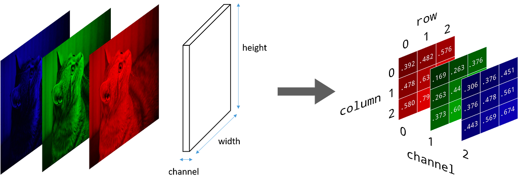
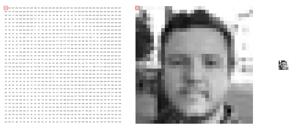
Input Matrix: An image is made up of pixels, where each pixel is in the inclusive range of [0, 255]. So we can represent an image, in terms of a matrix, where every position represents a pixel. The pixel value represents how bright it is, i.e. pixel -> 0 is black and pixel -> 255 is white (highest brightness). A grayscale image has a single matrix of pixels, i.e. it doesn't have any colour, whereas a coloured image (RGB) has 3 channels, and each channel represents its colour density.
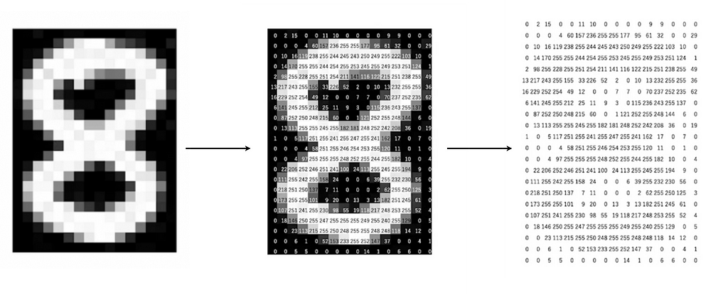
The above image is of shape: (24, 16) where height = 24 and width = 16. Similarly, we have a coloured image (RGB) having 3 channels and it can be represented in a matrix of shape: (height, width, channels)
Now, we know what is the first input to the convolution operator, but how to transform this input and get the output feature matrix. Here comes the term ‘kernel’ which acts on the input image to get the required output.
Kernel: In an image, we can say that a pixel surrounding another pixel has similar values. So to harness this property of the image we have kernels. A kernel is a small matrix that uses the power of localisation to extract the required features from the given image (input). Generally, a kernel is much smaller than the input image. We have different kernels for different tasks like blurring, sharpening or edge detection.
The convolution happens between the input image and the given kernel. It is the sliding dot product between the kernel and the localised section of the input image.

In the above image, for the first convolution, we will select a 3x3 region in the image (sequential order) and do a dot product with the kernel. Ta-da! This is the first convolution we did and we will move the region of interest, pixel by pixel(stride).
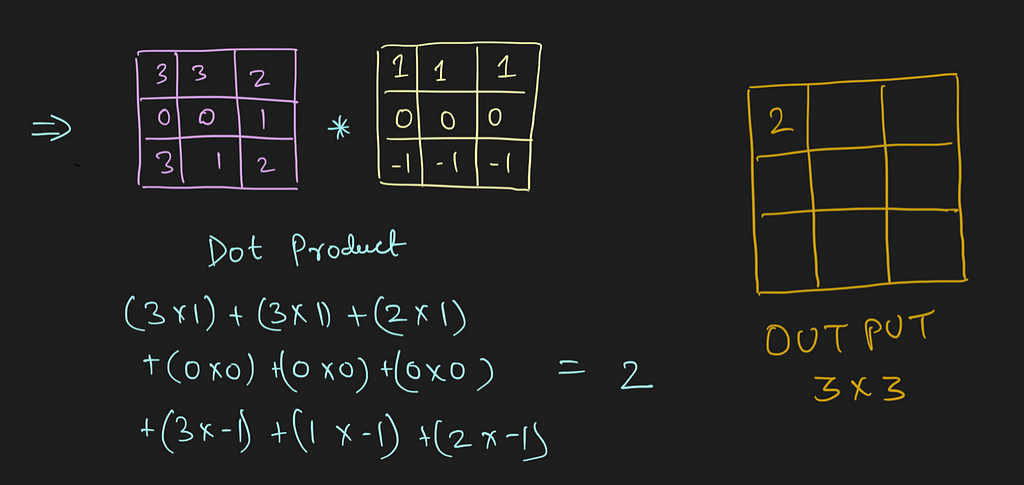
The dimension of the region of interest (ROI) is always equal to the kernel’s dimension. We move this ROI after every dot product and continue to do so until we have the complete output matrix.

So by now, we know how to perform a convolution, what exactly is the input, and what the kernel looks like. But after every dot product, we slide the ROI by some pixels (can skip 1, 2, 3 … pixels). This functionality is controlled by a parameter called stride.
Stride: It is a parameter which controls/modifies the amount of movement of the ROI in the image. The stride of greater than 1 is used to decrease the output dimension. Intuitively, it skips the overlap of a few pixels in every dot product, which leads to a decrease in the final shape of the output.

In the above image, we always move the ROI by 1 pixel and perform the dot product with the kernel. But if we increase the stride, let’s say stride = 2, then the output matrix would be of dimension -> 2 x 2 (Figure 8).
CONVOLUTION FOR MULTI-CHANNEL IMAGE
Now, we know what the input looks like, and what are some of the general parameters like kernel, and stride. But how does the convolution work if we have multiple channels in the image, i.e. image is coloured or to be more precise if the input matrix is of shape: (height, width, channels), where the channel is greater than 1.
Now you may have a question, we only have a single kernel and how to use it on a stack of the 2D matrices (in our case, three 2D matrices stacked together). So here we will introduce the term ‘filter’.
Generally people interchange filters and kernels, but in reality they are different.
Filter: It is a group of kernels which is used for the convolution of the image. For eg: in a coloured image we have 3 channels, and for each channel, we would have a kernel (to extract the features), and a group of such kernels is known as a filter. For a grayscale image (or a 2D matrix) the term filter is equal to a kernel. In a filter, all the kernels can be the same or different from each other. The specific kernel can be used to extract specific features.
So how does the convolution takes place?
Every channel is enacted by its kernel (exactly similar to convolution on a grayscaled image) to extract the features. All the kernels should have the same dimension. As a result, we have multiple output matrices (one each for a channel) combined (with the help of matrix addition) into a single output.
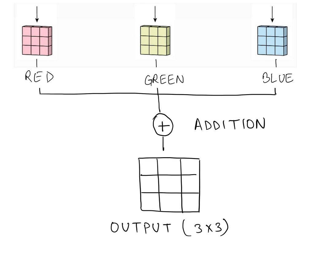
So the output is the feature map (extracted features) of the given image. We can further use this output with classical machine learning algorithms for classification/regression tasks, or this output can also be used as one of the variations in the given image.
PADDING & OUTPUT DIMENSIONS
At this juncture, we have a pretty decent understanding of how the convolution between the image and the kernels takes place. But this isn’t enough. Sometimes, there is a need to get the exact output dimension as that of the given input, we need to convert the input into a different form but the same size. Here comes the usage of padding.
Padding: It helps in keeping the constant output size, otherwise with the use of kernels, the output is a smaller dimension and could create a bottleneck in some scenarios. Also, padding helps in retaining the information at the border of the image. In padding, we pad the boundary of the image (the edges) with fake pixels. More often, we use zero-padding, i.e. adding dark pixels at the edges of the matrix, such that the information at the original edge pixels isn’t lost.

We can also add multiple padding, i.e. instead of a single-pixel pad at every edge, we can use n number of pixels at the boundary. This is normally decided by the kernel dimension used in the convolution.
Congratulations! We have covered the foundational concepts of convolution operation. But, how do we know the output shape of the matrix? And to answer this, we have a simple formula that helps in calculating the shape of the output matrix.

Where:
wᵢ -> width of the input image, hᵢ -> height of the input image
wₖ -> width of the kernel, hₖ -> height of the kernel
sᵥᵥ -> stride for width, sₕ -> stride for height
pᵥᵥ -> padding along the width of the image, pₕ -> padding along with the height of the image
Generally, the padding, stride and kernel in a convolution are symmetric (equal for height and width) which converts the above formula into:

Where:
i -> input shape (height = width)
k -> kernel shape
p -> padding along the edges of the image
s -> stride for the convolution (for sliding dot product)
So, now what? In the upcoming section, we are going to learn about different types of kernels, which are designed to perform a specific operation on the image.
IMAGE KERNELS
Convolutions can be used in two different ways; either with a learnable kernel in a Convolutional Neural Network with the help of gradient descent or with a pre-defined kernel to convert the given image. Today, we would be focusing on the latter one and learning what all different types of transformations are possible with the help of kernels.
Let’s consider this as an input image.
Now, with the help of kernels and using convolution on the input image and the given kernel, we would transform the given image into the required form. Following are a few transformations, that can be done with the help of custom kernels in image convolutions.
- Detecting Horizontal and Vertical lines
- Edge Detection
- Blur, sharpen, outline, emboss and various other transformations found in Photoshop
- Erode and Dilation
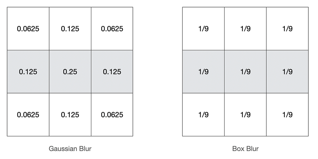
So let’s first have a look at one of the most basic kernels, and it is the blur kernel. There are many variations of the blur kernel, but the most famous are Gaussian and Box blur.

Similarly, other kernels help in the transformation of the image into its required form. We have a great illustration to try out different kernels on the above image: https://setosa.io/ev/image-kernels/
But generally, there are some kernels, that we as data scientists should get a hold of, and it is the line detection kernel which primarily includes horizontal, vertical and diagonal lines.
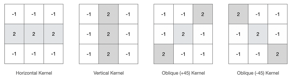
From the above graph, the intuition of these line detection kernels is very clear. Suppose the task is to detect horizontal lines in an image. Let’s construct a kernel for the same. So in general a 3 x 3 kernel is a good option to start with. Now to detect the horizontal lines (from the above intuition) what if we subtract all the nearby pixels considering it is a horizontal line. In that scenario, the horizontal line would be easily visible as we have decreased the pixel values in its vicinity, which would be in a straight line or precisely parallel to the type of line we wish to detect.
But in what ratio should we decrease the pixels in the vicinity or increase the pixel for the line to detect? Actually, it all depends on the use case along with a few iterations with the kernels, to get a good match.
Let’s play with the given horizontal kernel and its convolution results.
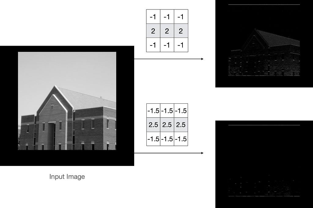
Surprised! So from figure 20, we can easily state that if we increase the values in the basic horizontal kernel, then only a few lines are detected. This is the power of kernels on the image. Moreover, we can also increase/decrease the density for the given kernel by symmetric modification of the given values.
This was it…Hope you learned and also loved the blog :D
CONCLUSION
In the given blog post, the following topics were discussed:
- Basic Terminologies of Convolution: Input, Kernel, Stride, Padding, Filters
- Difference between grayscale and coloured images
- 2D Convolution on Grayscale and Coloured images
- The shape of the output of the convolution operator
- Exploring different Image Kernels
In the upcoming tutorials, you will get to learn the in-depth working of CNN layers, forward and backward propagation of CNN layers, different types of CNN layers and a few state-of-the-art deep learning models used for extracting feature maps.
REFERENCES
[1] CS231n Convolutional Neural Networks for Visual Recognition, https://cs231n.github.io/convolutional-networks/
[2] Vincent Dumoulin, Francesco Visin, A guide to convolution arithmetic for deep learning, https://arxiv.org/abs/1603.07285
[3] Line Detection, https://en.wikipedia.org/wiki/Line_detection
[4] Irhum Shafkat, Intuitively Understanding Convolutions for Deep Learning, https://towardsdatascience.com/intuitively-understanding-convolutions-for-deep-learning-1f6f42faee1
[5] Victor Powell, Image Kernels, https://setosa.io/ev/image-kernels/
Computer Vision: Convolution Basics was originally published in Towards Data Science on Medium, where people are continuing the conversation by highlighting and responding to this story.
from Towards Data Science - Medium https://ift.tt/7ZIy9SB
via RiYo Analytics


No comments