https://ift.tt/HCPBxJr On how the object’s velocity is estimated when not measured Photo by Jure Zakotnik on Unsplash Introduction ...
On how the object’s velocity is estimated when not measured
Introduction
The Kalman filter is a complicated algorithm, and in most cases, people use it without fully understanding its equations.
When I started working with the Kalman filter I did the same. I read a bunch of tutorials that tried to intuitively explain the algorithm, but in doing so, neglected a crucial part regarding the role of the covariance matrix.
The product I was working on was a detection-based object tracker. In it, the Kalman filter is used to predict and update the location and velocity of an object given a video stream, and detections on each of the frames. At some point, we wanted to also account for the camera tilt and pan by adjusting the location of the object given the angles of movement. The object’s velocity, of course, should be unaffected by such camera motion.
But, when starting to implement this adjustment I realized that I don’t really understand how the velocity is even estimated. I assumed that somewhere in the process there is an explicit calculation of the velocity given the previous and current locations (velocity, in our case, is never directly measured). I also assumed that this velocity is treated in the same manner as the location. To my surprise, both assumptions turned out to be false.
This led me to a deep dive into the Kalman filter’s equations trying to figure out what exactly is going on as intuitively as possible but with no oversimplifications. This blog is a summation of what I’ve learned through this process.
As this is not an introductory blog, I am going to assume that you are acquainted with basic concepts from probability theory such as probability distribution functions, Gaussians, and Bayes’ theorem. Also, we will conduct some calculations using matrix multiplication and addition. So all the better if you are familiar with that as well.
Overview
The Kalman filter is an algorithm designed to estimate the values of measured variables over time, given continuous measurements of those variables and given the amount of uncertainty in those measurements. The Kalman filter also accounts for given relations between the estimated variables.
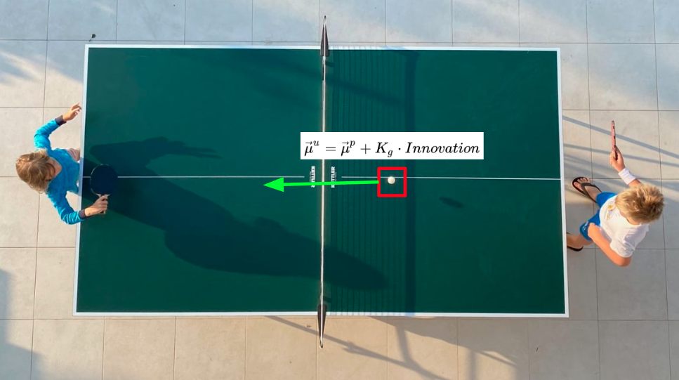
Let’s take as an example the process of tracking a ping-pong ball in a video, given 2D bounding box detections of the ball. The detections will likely contain some inaccuracies either in the coordinates of the given bbox or such caused by false positives/negatives.
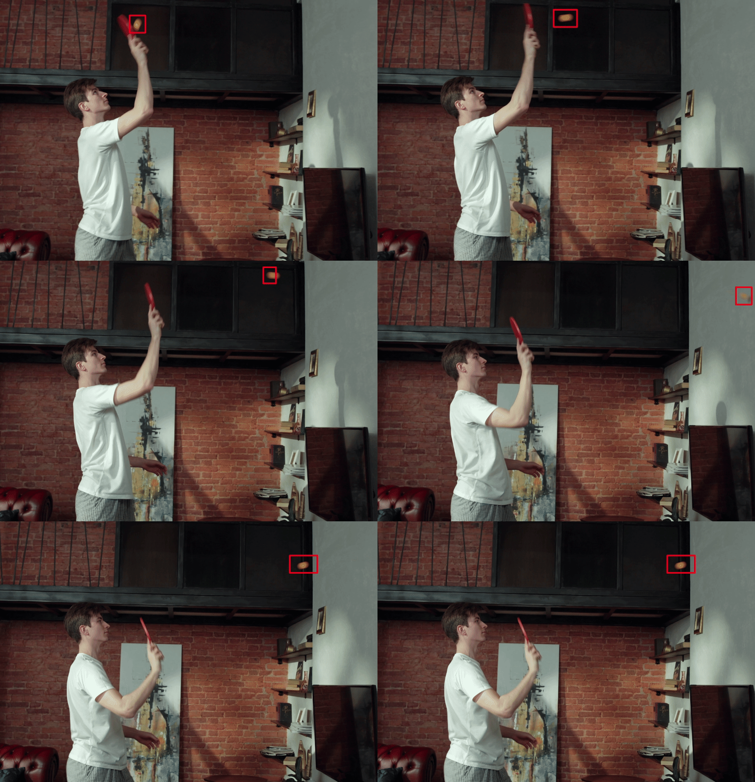
To track the ball more smoothly, we will want to track the measured center coordinate (x, y), width, and height of the bbox. Assuming that a moving ball’s velocity can be approximated as constant in short time intervals, we would also want to track the x and y velocities (v_x, v_y) to, hopefully, get these predictions:
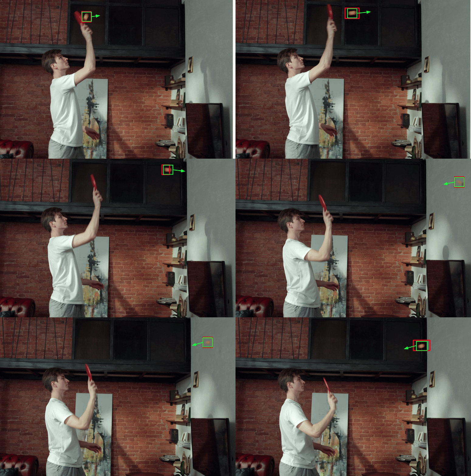
Usually, when trying to explain the Kalman filter, one would use an example of tracking an object using measurements for both its position and velocity (GPS and speedometer for example). In our example, we do not have a direct measurement of the velocity. Instead, the Kalman filter infers this velocity using the measured positions and prior knowledge we inject into its equations regarding the kinematic behavior we expect (a constant velocity in this case).
For simplicity, from now on we will only discuss the tracking of x and v_x (a 1D tracking example). After understanding what happens in 1D, the logic can be easily extended to 2 and 3 dimensions as each dimension is completely independent of the others in our example case.
The assumptions
There are two significant assumptions when using the Kalman filter:
- The sensor is noisy and its output and noise can be accurately modeled by a Gaussian probability distribution function (PDF).
- Our initial prior knowledge of the actual state is also a Gaussian PDF.
In our example, the sensor output is represented by a 1D Gaussian where the mean equals the actual sensor output and the variance is the sensor’s uncertainty (mostly measured empirically).
The prior Gaussian is two-dimensional (one for position and one for velocity). A 2D Gaussian can be completely described using 6 numbers: 2 for its center coordinate vector (a.k.a the mean), and 4 more for the 2x2 covariance matrix.
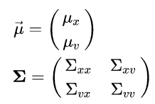
The diagonal of the covariance matrix corresponds to the variance of each dimension, and the 2 off-diagonal elements are the actual covariance between the position and velocity. The off-diagonal elements are always identical due to the symmetry of the covariance i.e. the correlation between x and y is the same as the correlation between y and x (we will get into more detail regarding this element later on).
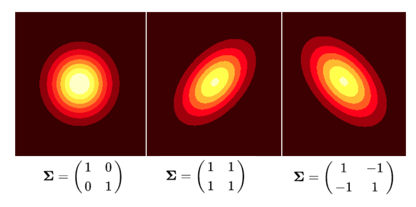
The Kalman filter will try to update the mean and the covariance using the input detections. The common terminology is to call this distribution the system state.
In our example, we will use the following initial state:
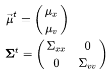
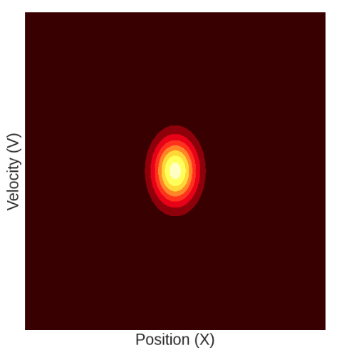
The mean position μ_x is taken from the x position of the first detected bbox, and we are assuming some initial velocity μ_v. We are also assuming that initially there is no covariance between the velocity and position. Graphically we can plot this initial state as follows:
The algorithm steps
To do its magic the Kalman filter has two steps: Predict, in which it tries to predict the current state given the previous state and the time that has passed since. Update, in which it tries to combine the predicted state with an incoming measurement. Let’s see how this happens using our example.
Predict step equations
To predict the next state given the time that passed, the Kalman filter uses a state-transition matrix (F), (a.k.a the physical model) which relates the previous state to the current one. In our case, as we are assuming constant velocity in short time intervals (in the order of a couple of frames), the state-transition matrix is:

Such that if we multiply it with our state mean vector we get the predicted mean:

Predicting the new mean is not enough. We expect that if time has passed then the covariance matrix (which represents the uncertainty of the state) would also change. To predict the new covariance, we will use the formula for a linear transformation of a random variable (see here for details) and also add to it a noise diagonal matrix. This noise is called “Process noise” and it encapsulates uncertainty created by the time that has passed since we last updated the state, and is not accounted for in our physical model. So in our example, it can represent non-constant velocities and camera movements. It is usually denoted by Q. So the covariance prediction equation is as follows:

If we solve this equation for our initial state:

Notice that apart from the extra uncertainty added by the process noise, the position variance also increased by a factor of:

This factor arises from the dependency between position and velocity we introduced when defining F (The physical model) as a non-diagonal matrix. It can be understood as follows: Given that the predicted position is a function of the state’s velocity, the uncertainty of this predicted position is the uncertainty of our previous state plus the uncertainty of the velocity times the factor by which they are coupled (squared, for units).
Another thing to notice here is the newly introduced covariance factor:

This means that our Gaussian dimensions are no longer independent. This is more easily explained graphically so let’s do that.
Predict step Intuition
Graphically, the update step looks like this:
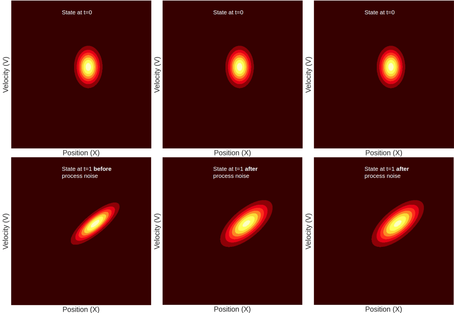
So what happened here? Why did our state suddenly shift sideways? This is because the position and the velocity are not two independent variables. The state’s velocity directly affects the predicted position. Intuitively, what this means is that higher velocity should correspond to a farther position and vice-versa. Mathematically, this is indicated by the fact that our state-transition matrix (F) is not diagonal. The off-diagonal element Δt is what couples together the position and the velocity.
Because of this coupling, each update step introduces off-diagonal elements in the covariance matrix which graphically correspond to the shifting of our distribution as shown in the GIF above.
Update step Intuition
This step is a bit more complicated mathematically, but intuitively it’s also very simple. In this step, the Kalman filter will receive as input two possible states (defined as Gaussian PDFs) and outputs a new state which combines the information from both.
Before diving into the equations that actually describe this process, here’s the gist: Combining information from two (or more) PDFs, in a statistically optimal way, is equivalent to multiplying them together. Because of a special property of Gaussian distributions, the product of this multiplication is yet another Gaussian distribution with mean and covariance that can be obtained with (relatively) simple equations.
Now for more details. The update process can be thought of as Bayesian inference. If we define the actual position of the object we are tracking (that we don’t actually know) as x and the actual measured position as m we get the following update equation:
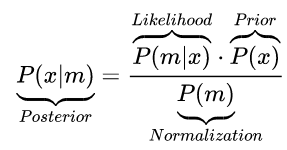
Let’s understand these terms in the context of the Kalman filter:
- Posterior: The probability distribution of the actual location, given the measurement. This is what we want to infer using the update step.
- Likelihood: The probability distribution of the measurement, given the state. This is assumed to be a Gaussian distribution around the actual position (as discussed in the “The assumptions” section).
- Prior: The probability distribution of the actual state to the best of our current knowledge prior to the measurement (a.k.a the predicted state). This is also assumed to be a Gaussian initially.
- Normalization: The measurement probability distribution, summed over all possible locations. In this context, this part is not calculated as we only care about updating the mean and covariance and don’t care about the Gaussians’ amplitudes.
From here we can deduce that the updated state will be a product of the predicted state and measured state (for more on likelihood functions check this blog out, and for a lot more on likelihood in Kalman filters check out chapter 4 of this book). Because we are dealing here with Gaussian distributions, the product of such distributions will be yet another Gaussian distribution with closed equations for its mean and covariance.
If we had measurements for both the position and the velocity (which we don’t) the update step would like something like this:
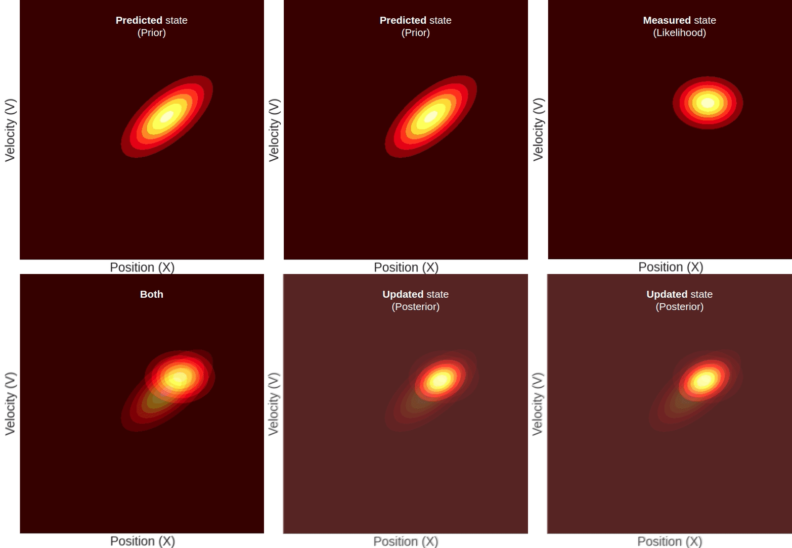
The predicted state is taken from the process depicted above. The measured state, similar to our initial state, has an axis-aligned oval shape. This is to say that the measured position and the measured velocity come from two independent sensors, with the uncertainty of each captured by the Gaussian’s variance.
But, because in our video tracking example, we only have a position measurement and no velocity measurement, the measured state’s probability will only decay in the position dimension, but in the velocity dimension, it will have a uniform distribution, so it will look something like this:
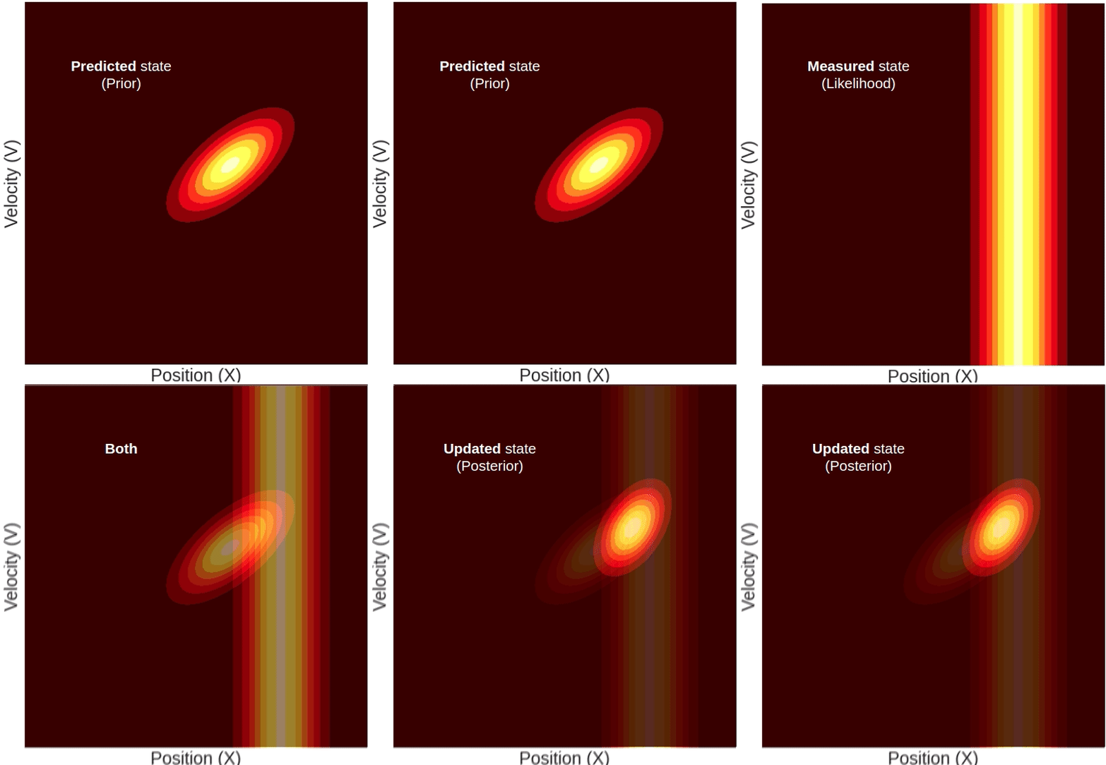
Here you can see a measured position that has a higher mean than the predicted one. The updated state’s position will, of course, be somewhere in between. But notice, although we only measured the position, the updated state’s mean velocity also increased with respect to the predicted state. This change in velocity can be understood intuitively if we recall that the predicted state’s position and velocity are correlated, meaning that farther locations are associated with higher velocities. Given this property, it becomes clear why measuring a certain position will result in a change in our belief about the mean velocity.
Think about two probability distributions that are highly correlated: the cloudiness probability distribution, and the amount of rain probability distribution, for example. We know that a high amount of clouds is highly correlated with more rain. Now say we had to guess how much rain fell yesterday in Paris. Without any prior knowledge, you would guess, let’s say, 3mm of rain (the mean of your guess). Now, someone tells you that yesterday was very cloudy. Using this prior knowledge you would definitely update your guess about the rain to a higher amount. This is exactly what happens in the Kalman filter. Given a far position measurement, we also update the velocity to a higher value.
Mean update equations
In this blog, we will not try to derive the “update” equations (for that you can look here) but rather we will just show them and try to make sense of them.
First of all some definitions:
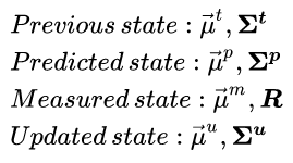
We are using R to represent the measured state covariance matrix as this is the common way to denote it in Kalman filter textbooks. In this example, as our measurement is 1D, the measured state can be represented by two scalars:

Because our measurement and state have different dimensionality, to combine the two, we need a linear transformation that takes us from the state space to the measured space. We denote this transformation with the matrix H. In our case, our measurement has only one dimension (the position) whereas the state has two (position & velocity), so to transform between them we can use:

That way, if we multiply our predicted mean with H we will get only the measured part of the mean:

Now for the actual equations. We will first give the full equations for the updated state’s mean and covariance and then break them down into more meaningful components so we can better understand what’s going on.
The full updated mean equation (for our 1D video tracking example) is:

This is a pretty complicated equation so let’s break it down. Firstly, we define the sensor “Innovation” as:

Which is simply the difference between the measured position and the mean predicted position. It’s called innovation because it can be thought of as the new (innovative) information that we get from the sensor.
Secondly, we define the “Kalman gain” as:
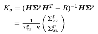
The Kalman gain is the factor by which we incorporate the new sensor information into the updated state.
Plugging these definitions into the equation we get:
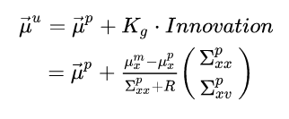
Let’s break this down further to the position update and the velocity update. For the updated position we get:
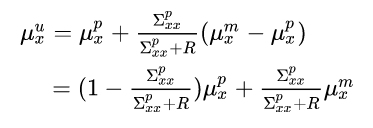
This equation makes a lot of sense. The updated mean will be a weighted average of the predicted and measured mean, with the weight factor being proportional to the relative uncertainty of each of them.
So let’s say we have a perfect sensor with zero variance. This will result in the predicted measurement being equal to the sensor measurement (as it should — It’s perfect.). On the other hand, if the sensor is very noisy (high uncertainty) compared to the predicted state’s variance then it will be the other way around, ignoring the measurement completely and only using the predicted position. Exactly as you would expect.
Now for the mean velocity update:

Not a lot of sense in this general form (at least not that I can think of) so let’s try plugging in the results for a single covariance prediction step we derived earlier and see if that helps. If we assume zero process noise (Q=0, which is unrealistic but good for easier and more intuitive equations) we get that the predicted covariance is:

Remember that the “t” superscript just means “of the previous step”; plugging into the velocity update we get:

We’ll multiply the numerator and denominator by Δt and get:

Let’s think about the different parts of this equation and what they entail. The last part:

is the velocity innovation. Just like the position innovation, this is the difference between the predicted state velocity and the velocity needed if we were to actually reach the measured position. Now, how much of this innovation do we want to be incorporated into the updated state? Well, it depends on the uncertainty of the velocity in our previous state relative to the uncertainty of the measured velocity. But wait, we didn’t measure the velocity! It was inferred from the position measurement. So how would we define the uncertainty of this inferred velocity?
The velocity was inferred using the previous position and the measured position so it makes sense that its uncertainty would be a sum of the uncertainty of its two components. So we can define the inferred velocity uncertainty as:

If we recall that:

we can also define a generalized predicted velocity uncertainty that also accounts for the time that passed since the last update as:

Plugging these definitions into the equation we get:

This equation is way more intuitive. What it is saying is that the updated velocity will equal the predicted velocity plus a fraction of the velocity innovation. This fraction will approach zero when the inferred velocity uncertainty is very large (relative to the predicted velocity), and approach 1 when it’s the other way around.
Covariance update equations
The full covariance update equation looks like this:

We can plug in the Kalman gain obtained above and the fact that:

to get:
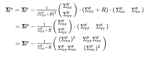
We’ll define the relative measurement uncertainty as:

This constant is just the measurement uncertainty relative to the total uncertainty in the position. If we plug this into the equation (after some more algebra that I will spare you) we get:
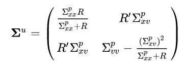
Let’s break this down: the updated position uncertainty is the harmonic mean of the predicted position uncertainty and the measured position uncertainty. A harmonic mean is a type of mean that combines two elements by approaching the smaller of the two elements. So if:

then:

and vice-versa.
The updated position-velocity covariance is also intuitive. It is a scaled-down version of the predicted covariance, with the scale factor being the relative measurement uncertainty. So, again, for a perfect measurement, these elements will approach zero, and for a noisy measurement, they will remain the same.
Now for the updated velocity variance. At first glance, it doesn’t seem to make much sense so, as we did before, let’s plug in the results for a single covariance prediction step we derived earlier.
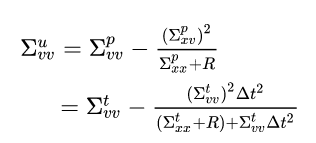
We can again use the inferred velocity uncertainty and the generalized velocity prediction uncertainty we defined above to get:

Again we get that the updated variance is the harmonic mean of the inferred velocity uncertainty and the generalized velocity prediction uncertainty. So basically always approaching the smaller of the two.
Finally, we have:
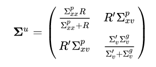
Let’s sum up what we can learn from this equation. Both the position variance and velocity variance can be expressed as harmonic means of two uncertainties (each with the ones associated with it). The position-velocity covariance also gets scaled-down as a function of how certain we are of measurement relative to the prior. If you go back to the graphic that shows the update process, this is also pretty intuitive why.
Summing up
In this blog, I tried to put into writing the process I went through trying to get an intuitive understanding of the Kalman filter’s equations. It was a mixture of graphical and mathematical intuitions which, in my view, complement each other. Hope it helped you get a better understanding of what is actually going on “under the hood” and that maybe now this complicated algorithm is a bit more approachable.
One point to add here is that algorithms such as object tracking should not be taken lightly. These algorithms, in the wrong hands, can be used to commit civil rights offenses and as such should only be developed by professionals and with high regulation.
What I Was Missing While Using The Kalman Filter For Object Tracking was originally published in Towards Data Science on Medium, where people are continuing the conversation by highlighting and responding to this story.
from Towards Data Science - Medium https://ift.tt/YTAjWKU
via RiYo Analytics

No comments