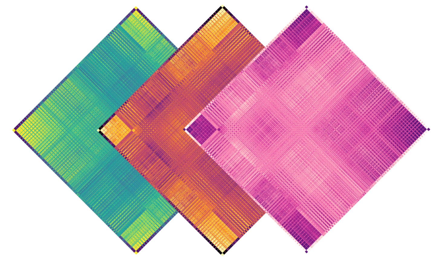
https://ift.tt/DSZh5s8 An aesthetic point-of-entry into recurrent neural network models Fig 1. assorted ‘memory’ matrices, corresponding ...
An aesthetic point-of-entry into recurrent neural network models
— OVERVIEW —
This article covers Hopfield Networks — recurrent neural networks capable of storing and retrieving multiple memories. We’ll begin with an in-depth conceptual overview, then move to an implementation of Hopfield Networks from scratch in python; here we’ll construct, train, animate, and track various statistics of our network. Finally, we’ll end with examples of the usage of Hopfield Networks in modern-day machine learning problems. Feel free to use the table of contents below to skip to whichever sections are pertinent to your interests. Please reach out if you discover any errors or inconsistencies in this work, or with feedback about how articles such as these can be improved for the future; thank you for your interest!
— TABLE OF CONTENTS —
- INTRO
- CONCEPTUAL BACKGROUND
- ENERGY PROOF
- CODE IMPLEMENTATION
- APPLICATIONS OF MODERN HOPFIELD NETWORKS
- HELPFUL LINKS
— INTRO —
During every moment of your life, waves of activity propagate across the networks of your brain. Billions of signals continuously harmonize and oscillate; these networks are the functional architecture which underlie your everything. They are your love, your stress, your favorite song, and your hopes and dreams. Your entire sense of being and experience is formed from the dynamic behavior of these networks, held stable by memory systems which constantly adapt to better represent your place in an ever-changing environment.
The sheer scope and integration of networks in the human brain make it incredibly difficult to study how, where, or even if computation in the forms we’re familiar with occurs. There is evidence for information processing at the levels of modulatory proteins in single cells, cortical microcircuits, and brain-wide functional networks, among others. Experimental understanding of the brain moves slowly. Fortunately, clever engineers have invented or discovered algorithms which can, in part, model aspects of these networks. No single model will ever encapsulate the absolute complexity and behavior of the human brain, but these tools allow students of such systems a convenient window to observe the ways in which information might be computed, and ultimately represented, within the activity of a distributed network.
For the purpose of this writeup, we will be analyzing and implementing binary Hopfield neural networks in python. Though newer algorithms exist, this simple machine is both an informative and aesthetically pleasing point of entry into the study and modeling of memory and information processing in neural networks. We’ll begin with conceptual background, then move to implementation. Finally we’ll cover some functional use-cases for Hopfield Networks in modern data analysis and model generation.
— CONCEPTUAL BACKGROUND —
Hopfield networks are a beautiful form of Recurrent Artificial Neural Networks (RNNs), first described by John Hopfield in his 1982 paper titled: “Neural networks and physical systems with emergent collective computational abilities.” Notably, Hopfield Networks were the first instance of associative neural networks: RNN architectures which are capable of producing an emergent associative memory. Associative memory, or content-addressable memory, is a system in which a memory recall is initiated by the associability of an input pattern to a memorized one. In other words, associative memory allows for the retrieval and completion of a memory using only an incomplete or noisy portion of it. As an example, a person might hear a song they like and be ‘brought back’ to the memory of their first time hearing it. The context, people, surroundings, and emotions in that memory can be retrieved via subsequent exposure to only a portion of the original stimulus: the song alone. These features of Hopfield Networks (HNs) made them a good candidate for early computational models of human associative memory, and marked the beginning of a new era in neural computation and modeling.
Hopfield’s unique network architecture was based on the Ising model, a physics model that explains the emergent behavior of the magnetic fields produced by ferromagnetic materials. The model is usually described as a flat graph, where nodes represent magnetic dipole moments of regular repeating arrangements. Each node can occupy one of two states (i.e. spin up or spin down, +1 or -1), and the agreement of states between adjacent nodes is energetically favorable. As each dipole ‘flips’, or evolves to find local energetic minima, the whole material trends toward a steady-state, or global energy minimum. HNs can be thought of in a similar way where the network is represented as a 2D graph and each node (or neuron) occupies one of two states: active or inactive. Like Ising models, the dynamic behavior of a HN is ultimately determined according to a metaphorical notion of ‘system energy’, and the network converges to a state of ‘energetic minimum’, which in the case of a learned network happens to be a memory.
In order to understand the layout and function of a Hopfield Network, it’s useful to break down the qualities and attributes of the individual unit/neuron.
Each neuron in the network has three qualities to consider:
connections to other neurons — each neuron in the network is connected to all other neurons, and each connection has a unique strength, or weight, analogous to the strength of a synapse. These connection strengths are stored inside a matrix of weights.
activation — this is computed via the net input from other neurons and their respective connection weights, loosely analogous to the membrane potential of a neuron. The activation takes on a single scalar value.
bipolar state — this is the output of the neuron, computed using the neuron’s activation and a thresholding function, analogous to a neuron’s ‘firing state.’ In this case, -1 and +1.
The information, or memories of a Hopfield Network are stored in the strength of connections between neurons, much in the same way that information is thought to be stored in the brain according to models of long term memory. The connections, and their respective weights, directly affect the activity of the network with each generation, and ultimately determine the state to which the network converges. You can picture the weight between 2 neurons, neuron-a and neuron-b, as the extent to which the output of neuron-a will contribute to the activation of neuron-b, and vice versa. More on activation and its effect on neuronal state below.
Importantly, the connections between neurons in a HN are symmetric. This means that if neuron-a is connected to neuron-b with a strength of +1, neuron-b’s connection to neuron-a is also +1. We can store the weights of a network with n neurons in a square symmetric matrix of dimensions n x n. Because neurons do not connect back to themselves, the weights on the matrix’s diagonal are effectively null. It’s important to note that the network structure, including the number of neurons and their connections in the network, is fixed. The weights of those connections are the tunable parameter. When we speak of ‘network learning’ what we really mean is the fine-tuning of each weight in the network in order to achieve some desirable output. In the case of an HN, the initial state configuration can be thought of as an input, and its final state configuration as the output. Because each neuron is updated depending on linear combinations of its inputs, the entire network is really one massive mathematical function: a dynamical system, which, with each update generation, takes its past output as its current input. The parameters of this function, the weights, determine the way the network evolves over time.
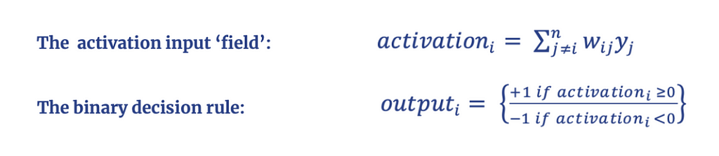
Any neuron’s instantaneous activation can be calculated by taking the weighted sum of inputs from the neurons it’s connected to:
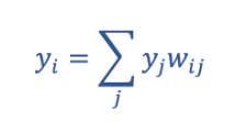
Where yi represents the activation of neuron-i in the network, yj represents a vector of the respective outputs of all neurons inputting to neuron-i, and wij the symmetric weight of the connection between neurons i and j.
The activation of a neuron is used to determine the state, or output, of the neuron according to a thresholding function:
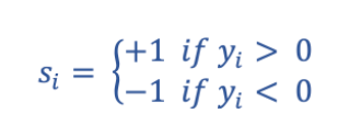
Where si represents a neuron-i’s given state and output.
As the state of each neuron in the network is updated, its contributions to the activities of other neurons change; this in turn feeds back and modulates more activity, and so on, until the network reaches a stable formation. If a neuron’s activation during a given generation is positive, its output will be +1 and vice versa. Another way to think of this is that a given neuron is receiving a ‘field’ of inputs analogous to its activation. Each and every input the neuron receives is weighted, and summed, to yield a net activation, be it positive or negative. If the sign of that field differs from the sign of the neuron’s current output, its state will flip to align itself. If the sign of the field of input matches the sign of the neuron’s current output, it will stay the same. If we consider the behavior of the overall network according to these rules, the quality of recurrence becomes clear; each network update, or output, becomes the input for the next timestep.
Now we’ve defined the characteristics of single units, but how does this translate to the distributed storage and representation of information in the network?
While each neuron can represent one of two states at a given time, the overall state of the network, termed s, can represent a string of binary information. Take this pattern for example:
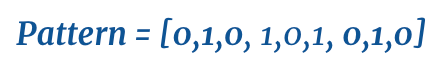
This pattern is a 1 x 9 binary vector which can be reshaped to a 3 x 3 matrix:
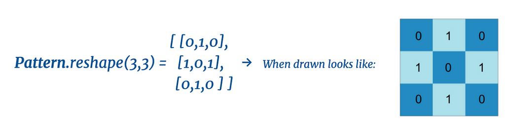
An image is just a matrix of numerical pixel values, so any image which can be represented with pixel values occupying binary states can be accurately represented by the states of a binary HN. Many forms of information can be represented in a binary/bipolar fashion, but we will focus on images as our use-case.
If a pattern takes the form of an image, we represent the pixels themselves using individual neurons. In the example above we have a 3 x 3 matrix of pixels, so we require 9 neurons to fully represent the image. Another way to visualize this is to represent the network as a graph, as shown below:
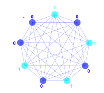
In this network graph, the nodes represent neurons and the edges represent the connections between them. The red dot indicates the neuron whose state represents the first element ,1, in the pattern vector. Following the state of the neurons in clockwise order yields the rest of the pattern.
In a computer, the state of each neuron is represented as the individual elements in a 1 x 9 vector, S. In other words, we directly represent the information we are trying to store using the respective states of neurons in the network:
S = [0,1,0 ,1,0,1, 0,1,0].
Any arbitrary information string of n bits can be represented by a network of n neurons. It is the combined activity of the neurons in the network which collectively represent our target information in a distributed fashion. In most HNs, the states of neurons are bipolar (-1 or +1). For the sake of simplicity, the example above uses binary 0 or 1, from here on out assume that the neurons occupy bipolar states.
Now that we know how the states of neurons are updated over time, and how the states themselves represent binary information, we get to the real ~magic~ of Hopfield Networks: their evolution towards a memorized pattern.
Here, a bit more background information is helpful. HNs are often called ‘attractor networks,’ because they tend to evolve to, or are attracted to, a “steady state”. To see this in action, let’s consider again the example pattern above. For the purpose of this section, assume the network has already learned the pattern (we’ll get into the details of learning in a little bit). Say we initialize the network to a random state, and let the network run according to the update rules described above, one neuron at a time:
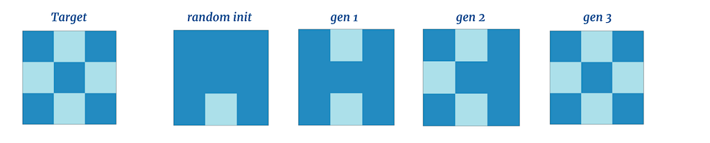
Here we see that despite the network’s randomly initialized state, it was able to restore the target memory in just three update generation steps — the overall state of the network was attracted to the memory state. Let’s bump the resolution of our target patterns up a notch:
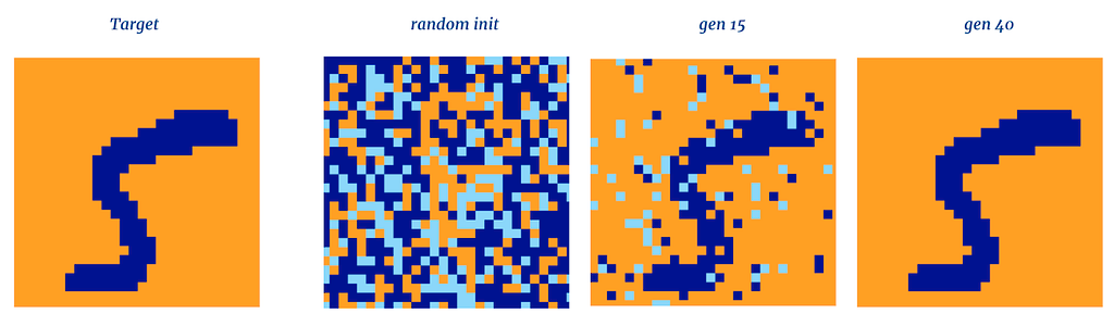
Incredible! Once again, the network slowly converges to a steady state, in this case a hand-drawn ‘5’, and does not update further. This behavior is significant. Despite each neuron’s initial state being scrambled, the weights of the connections between the neurons, along with their respective activations and outputs, are sufficient to push the overall network state closer to the memorized pattern with each subsequent update. Each neuron knows only its own state and incoming inputs, and yet a distributed pattern emerges from the network’s collective activity.
Networks configured in this way are actually capable of storing up to ~0.14n patterns, where n is the number of neurons in the network. When multiple patterns are stored, the network will converge to whichever pattern is most similar to the network’s initial state. An example of multiple stored patterns is shown below.
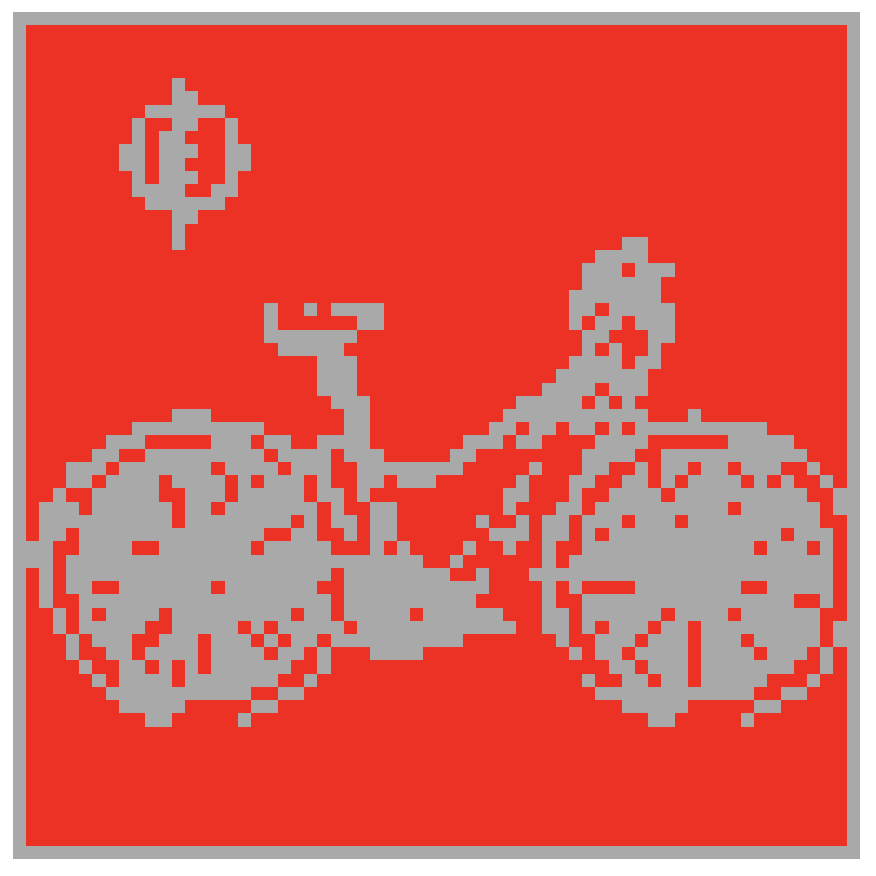
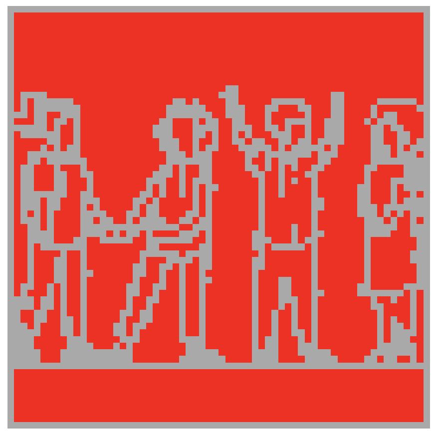
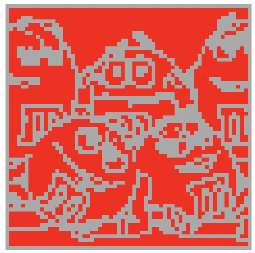
In the example above, the same 4096-neuron neural network has memorized three distinct patterns (the red images). Each pattern is a 64x64 pixel image learned by the network. The network is subsequently initialized three separate times from a distorted version of each image. During each update generation, 256 neurons (7.2% of the network) are randomly chosen and updated according to the binary threshold update rule. Although each network initialization is heavily distorted, the network restores each respective pattern as its state converges. Through learning of several patterns, the network has become capable of flexible, stimulus-specific behavior!
In these example memories, the information that we recognize are the simple spatial relationships of lit and unlit pixels, i.e. shapes, which make an image recognizable. However, any information which can be stored as a string of binary values can be memorized and recalled by a HN. A later section of the post will discuss state-of-the-art applications of HNs, but for imagination’s sake, let’s go back to the example from the intro: Imagine that the state of a very high-dimensional and integrated attractor network in your brain is encoding many pieces of information regarding the sensory and contextual circumstances under which you heard your favorite song for the first time, i.e. a memory.
Who you were with, your immediate surroundings, your emotional valence during the experience, etc… Although these pieces of information encode different parts of the memory, they might be recalled all at once by the same memory network when you later hear the song by itself. This phenomenon is known as pattern completion and is an entire subarea within the study of human memory. The physical mechanism is thought by some to be mediated by the presence of attractor dynamics in the human hippocampus — see this excerpt from The mechanisms for pattern completion and pattern separation in the hippocampus Rolls, 2013 :
Many of the synapses (connections) in the hippocampus show associative modification as shown by long-term potentiation, and this synaptic modification appears to be involved in learning (see Morris, 1989, 2003; Morris et al., 2003; Nakazawa et al., 2003, 2004; Lynch, 2004; Andersen et al., 2007; Wang and Morris, 2010; Jackson, 2013). On the basis of the evidence summarized above, Rolls (1987, 1989a,b,c, 1990a,b, 1991) and others (McNaughton and Morris, 1987; Levy, 1989; McNaughton, 1991) have suggested that the CA3 stage acts as an autoassociation [also called attractor] memory which enables episodic memories to be formed and stored in the CA3 network, and that subsequently the extensive recurrent connectivity allows for the retrieval of a whole representation to be initiated by the activation of some small part of the same representation (the recall cue).
Before we jump into a python implementation of HNs, there are two network-level concepts which go hand-in-hand that are useful to understand:
- Network learning — The computation of network weights which will enable the network’s state to evolve toward one or more memory attractors
- Network Energy — A mathematical basis and useful analogy which helps to understand why the network is guaranteed to converge to an attractor state, or energetic minimum.
First, let’s take a look at the weights matrix for the 4096-neuron network shown above:
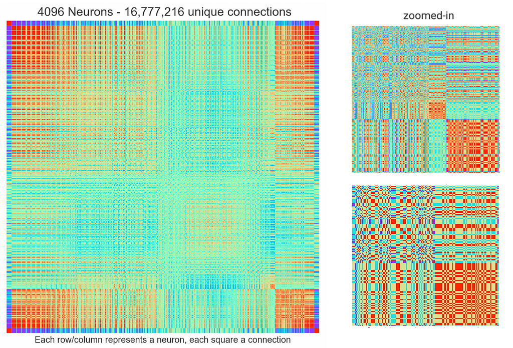
The first thing you should notice is that this graph looks very cool ;). Each row/column represents a neuron, and the intersections between rows/columns represents a color-coded connection weight. The second thing you should notice is that we have a diagonally symmetric matrix. This is to be expected, as the colored intersections between rows/columns are representing weights of symmetric and bi-directional connections that we discussed previously. Technically, we only need one half of this square, but a symmetric array like the one above is easier to calculate and implement in a computer, and it’s much more fun to look at.
We now know that the weights of the network’s connections are what determine its attractor dynamics. So the million dollar question is: how do we engineer these weights so that the network has an attractor for each memory we desire it to remember?
There are several learning algorithms known to be useful for HNs, but here we’ll be utilizing hebbian learning. The hebbian learning algorithm originates as a rule to describe the phenomenon of synaptic plasticity in biological neural networks. Taken generally, hebbian learning can be condensed to the statement that ‘neurons which fire together, wire together’. In other words, if two neurons which are connected via synapse are active at the same time, their connection strength increases (in the case of HNs, more positive), and their activity becomes more correlated over time.
The opposite is true for neurons which fire asynchronously, and instead their connection weights decrease (in the case of HNs, become more negative). In our example of stored images, the intuition behind Hebbian learning is clear. We want the weight between neurons which are either simultaneously ‘lit’ or ‘unlit’, in the target pattern to encourage the alignment of their activity as the network is updated. We also want cells whose states oppose each other to have the opposite behavior.
The formula to calculate a single weight between two neurons, i and j, according to hebbian learning is given by:

Where si and sj are the respective states that the neurons i and j will take on in the target pattern. To compute weights which result in several simultaneously-stored patterns, the formula is expanded…:
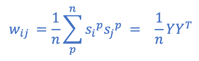
…which effectively takes the average computed weight across patterns, where p represents any pattern and n the number of patterns. On the right side, we have the equivalent expression in matrix form, where Y is a matrix containing our patterns as row vectors. Importantly, when storing multiple patterns, the number of bits in each pattern must remain consistent when the network is learning via this algorithm.
As previously mentioned, one significant feature of learning in this way is that it is ‘one-shot’, meaning that the network requires only one ‘exposure’ to learn. This is because we compute the entirety of the weights matrix in one operation. One-shot learning is somewhat unique in that it directly contrasts modern deep learning via backpropagation; a process characterized by iteratively adjusting network weights to reduce a classification error signal. Depending on the task, training via backpropagation often requires tens of thousands, or even millions, of training examples. This makes it a poor candidate as a model for human episodic memory processing which, by definition, requires one ‘episode’ for memorization. Interestingly, the hippocampus, an area known to have attractor-like dynamics, is actively recruited during one-shot learning, and sparse ensembles in this area are known to coordinate the recapitulation of past-cortical states during episodic memory recall.
It’s beyond interesting to me that functional and architectural symmetries exist between what have been observed in biological networks in-vivo, and the behavior of attractor networks in-silico. To me, this suggests that the underlying mechanisms behind such behaviors as memory, cognition, and learning, may be more ‘fundamental’ than the systems by which they’re physically instantiated, whether it be the brain or CPU, etc…
Up to now we’ve covered HN structure, behavior, and learning. Next, we tie everything together and understand why HNs behave the way they do using the notion of network energy.
We know that regardless of the initial state of an HN, it trends toward a ‘fixed-point’ attractor in state-space. ‘Fixed point’ is one way of describing that the network state remains steady, i.e. the network could update forever at this point and no neurons would flip. This phenomenon is not foreign to us; we commonly observe systems which converge to steady states. Consider a ball rolling down a hill until it sits at the bottom, or a dropped coin spinning rapidly on the ground until it rests stationary on one of its sides. The states of such systems, which you could describe as the objects’ positions, velocities, etc, converge to configurations which do not change without further perturbation. Using the Ising model as an example, the orientations of magnetic dipoles in a high-temperature magnetic material might be in a highly entropic, disordered state. If the material were allowed to cool, the dipoles would independently align to their local fields, and the entire material would tend toward a homogenous and steady globally-aligned state. The commonality between these examples is that their final states rest in energetic minima. In other words, it is thermodynamically favorable for them to come to rest, so from the moment each system’s external perturbations cease, they begin their respective state-trajectories toward the lowest energy possible.
HNs implemented in the computer are not physical systems which evolve toward thermodynamically-stable states. However, because of the constraints built into the network, defined by their structure and update rules, they display analogous behavior. Remember, they were initially inspired by the Ising model.
In fact, HNs have a scalar value, termed Energy, which monotonically decreases with each subsequent update generation. A HN’s state-trajectory over time can be thought of as a point descending an energy landscape; when the network converges to a memory, it has found itself in a ‘valley’ of the landscape, and will evolve no further unless disturbed.
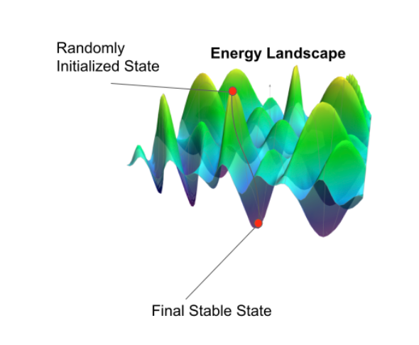
The beauty of HNs lies in the fact that, depending on learned weights, the respective attractors, or energetic minima, are adjustable. Any state of the system can be made, or learned, to be an attractor, and thus any state can be a learned memory. Below is a mathematical description of Energy in HNs, showing how Energy is guaranteed to decrease over subsequent update generations.
— Hopfield Energy Proof —
Note: The proof below is by the author and is based on mathematics presented in a lecture on Hopfield Networks by Carnegie Mellon)
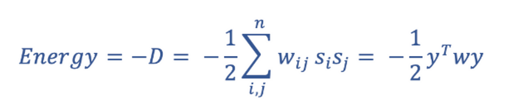
I find it useful to think about Energy in this context as a tension, as it fits nicely with the concept of physical energy. The Energy of a network is computed by multiplying the respective states of every neuron pair by each other, as well as the connection weight between them, and then summing this value across all possible pairs:
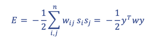
The key takeaway here is that the tension, or network Energy, is highest when the states of individual nodes do not agree with their incoming ‘input field’. The binary update rule relieves this tension by aligning the signs of a neuron’s output and its incoming input field, and in doing so each update generation reduces the global Energy of the network.
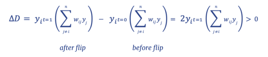
A neuron will flip when the sign of the product between its state and its input field is negative:

The state of a flipping neuron at t=1(post-flip) and t=0(pre-flip) are related by the expression:
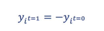
For instance, if the neuron was at state -1 at t=0, the flipped state would be +1 at t=1 and vice versa. According to these rules, there is a quantity associated with each flip that is guaranteed to increase. We nickname this quantity D and take the negative (-D) as our analogy for system energy, as this behavior more closely resembles the behavior of physical systems with energy.
So -D is guaranteed to decrease every generation, we sum -D across all neurons updated in each generation and term it Energy:
Okay, let’s see it in action!
Let’s initialize a trained HN to a distorted version of its memory, and compute this value E for each update generation as it is remembered. We expect to see that Energy is highest at the initialization, and lowest at the memory:

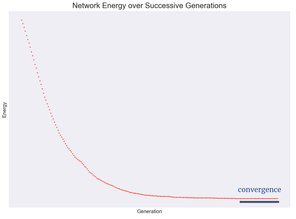
Here we see the decrease in E over subsequent update generations while the network remembers a picture of a butterfly. The portion of the graph marked ‘convergence’ is static as each and every neuron in the network agrees in state to the sign of its respective inputs. At this point, the network state matches the learned image and has thus converged to its memory.
— CODE IMPLEMENTATION —
We’ve covered the basics of Hopfield Networks; now it’s time to implement one from scratch in python.
This program will contain methods to build, train, and animate Hopfield Networks. We’ll import the MNIST handwritten digits dataset to use as an experiment. First we implement the core structure and essential functions of the network:
Next, we can conduct an experiment using samples taken from the MNIST handwritten digits dataset. We’ll pick a random digit as our network’s memory, and then animate the network’s update steps using pygame.
The fetch_MNIST function was written by George Hotz and can be sourced here.
There we have it! A fully functioning and animated HN. The code above provides an opportunity to explore these special networks’ behavior using image-memories.
— Applications of Modern Hopfield Networks —
If you’ve made it this far, you understand that the HNs which we’ve discussed thus far have neurons which occupy discrete binary states: -1 or 1. This is useful, but somewhat restrictive in terms of what information is possible to be efficiently stored within the network. Theoretically, a sufficiently large binary HN could store any information, but consider how many neurons you’d need to store even just one greyscale image.
Say we had a 28x28 image in grayscale; grayscale is an image format which stores pixel values as integers between 0(black) and 255(white). If we have 28x28 = 784 pixels in our relatively small image, and we choose to represent each pixel’s grayscale value as an unsigned 8-bit integer, we’d require a HN with 6,272 neurons to fully represent the informational content of the image. For a larger image resolution, say 1,024x1,024, we’d need >8,000,000 neurons. Information in modern-day machine learning is rich in both content and dimension, and so its clearly an advantage to have neurons which can occupy continuous states, decreasing the number of neurons needed to represent memories, and vastly increasing the informational storage capacity of the network.
Progress in the realm of continuous Hopfield Networks (CHNs) was introduced first in the 2020 paper Hopfield Networks is All You Need. CHNs offer a couple of advantages over classic binary HNs. As suggested by their name, the state of neurons in a CHNs are continuous, i.e. they are floats, rather than integers 0 or 1. So the state of a CHN at any given update generation is a vector of floating point numbers. This drastically increases the complexity of patterns which can be learned and retrieved by the network. In addition, the storage capacity of the network, as in how many distinct patterns it can remember and recall, is exponentially higher than in binary networks — binary Hopfield networks (BHNs) are prone to ‘spurious’ minima. If memories learned by a BHN are too similar, or if too many pattern vectors are learned, the network risks converging to an in-between memory, some combination of learned patterns; in other words, the network will fail to discriminate between patterns and becomes useless.
In 2020 paper cited above, the authors propose a CHN architecture which offers some applicability to modern-day machine learning problems. Notably, the network proposed:
- converges in one step
- stores exponentially more patterns than a BHN
- is capable of aiding in classification tasks with rich and high-dimensional data
I won’t cover the details of the paper here, but feel free to explore it yourself. The authors provide a use-case for their implementation, and show that, as a supplemental layer to a deep-learning architecture, CHNs perform better than other state-of-the-art algorithms in the complex task of immune repertoire classification.
All the code I used and a bit more can be found at this github repo. Below are some links which helped me tremendously when learning about Hopfield Networks!
— Helpful links —
- MIT opencourseware, Hopfield Networks
- Carnegie Melon Lectures on Hopfield Networks and Deep Learning
- Geoff Hinton Lecture on Hopfield Networks
- Interview with John Hopfield, creator of Hopfield Networks
- geeksforgeeks Hopfield Networks
- Yannic Kilcher explanation of Hopfield Networks is All you Need
Thank you for reading, and I appreciate any feedback!
Hopfield Networks: Neural Memory Machines was originally published in Towards Data Science on Medium, where people are continuing the conversation by highlighting and responding to this story.
from Towards Data Science - Medium https://ift.tt/c2Y4zL6
via RiYo Analytics


No comments