https://ift.tt/DtKWeub Recent Advances in Graph ML Recipes for cooking the best graph transformers In 2021, graph transformers (GT) won r...
Recent Advances in Graph ML
Recipes for cooking the best graph transformers
In 2021, graph transformers (GT) won recent molecular property prediction challenges thanks to alleviating many issues pertaining to vanilla message passing GNNs. Here, we try to organize numerous freshly developed GT models into a single GraphGPS framework to enable general, powerful, and scalable graph transformers with linear complexity for all types of Graph ML tasks. Turns out, just a well-tuned GT is enough to show SOTA results on many practical tasks!
This post was written together with Ladislav Rampášek, Dominique Beaini, and Vijay Prakash Dwivedi and is based on the paper Recipe for a General, Powerful, Scalable Graph Transformer (2022) by Rampášek et al. You can also follow me, Ladislav, Vijay, and Dominique on Twitter.
Outline:
- Message Passing GNNs vs Graph Transformers
- Pros, Cons, and Variety of Graph Transformers
- The GraphGPS framework
- General: The Blueprint
- Powerful: Structural and Positional Features
- Scalable: Linear Transformers
- Recipe time — how to get the best out of your GT
Message Passing GNNs vs Graph Transformers
Message passing GNNs (conventionally analyzed from the Weisfeiler-Leman perspective) notoriously suffer from over-smoothing (increasing the number of GNN layers, the features tend to converge to the same value), over-squashing (losing information when trying to aggregate messages from many neighbors into a single vector), and perhaps most importantly, poor capturing of long-range dependencies which is noticeable already on small but sparse molecular graphs.
Today, we know many ways to break through the glass ceiling of message passing — including higher-order GNNs, better understanding of graph topology, diffusion models, graph rewiring, and graph transformers!
Whereas in the message passing scheme a node’s update is a function over its neighbors, in GTs, a node’s update is a function of all nodes in a graph (thanks to the self-attention mechanism in the Transformer layer). That is, an input to a GT instance is the whole graph.
Pros and Cons of Graph Transformers
Feeding the whole graph into the Transformer layer brings several immediate benefits and drawbacks.
✅ Pros:
- Akin to graph rewiring, we now decouple the node update procedure from the graph structure.
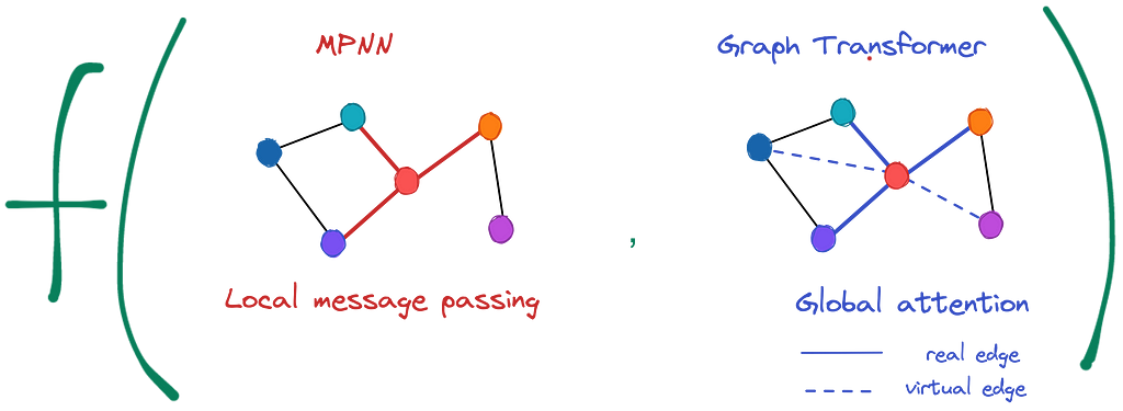
- No problem handling long-range connections as all nodes are now connected to each other (we often separate true edges coming from the original graph and virtual edges added when computing the attention matrix — check the illustration above where solid lines denote real edges and dashed lines — virtual ones).
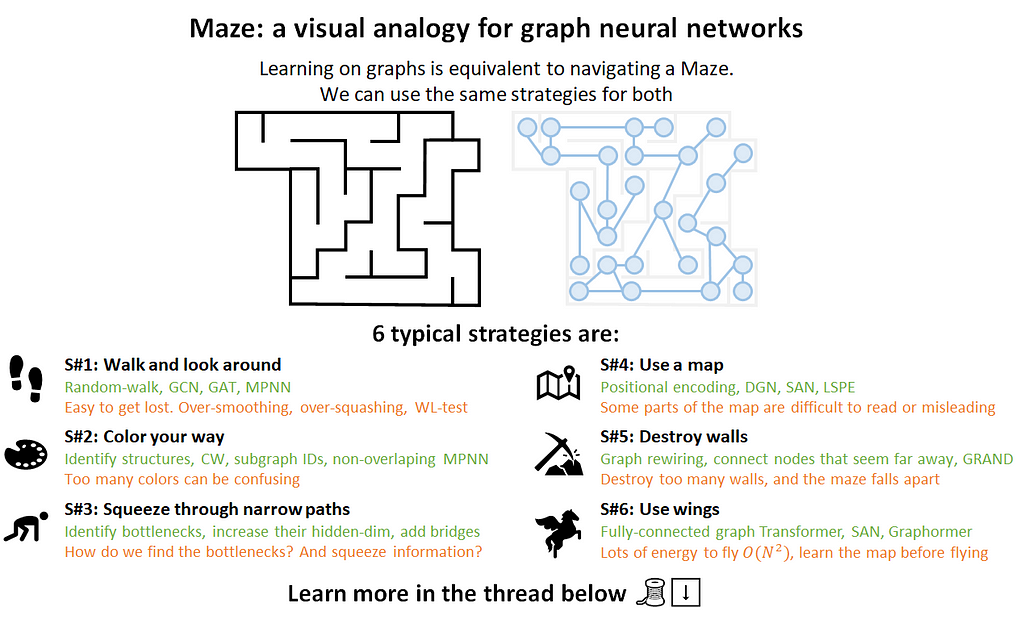
- Bringing the “Navigating a Maze” analogy, instead of walking and looking around, we can use a map, destroy maze walls, and use magic wings 🦋. We have to learn the map beforehand though, and later we’ll see how to make the navigation more precise and efficient.
🛑 The cons are similar to those stemming from using transformers in NLP:
- Whereas language input is sequential, graphs are permutation-invariant to node ordering. We need better identifiability of nodes in a graph — this is often achieved through some form of positional features. For instance, in NLP, the original Transformer uses sinusoidal positional features for the absolute position of a token in a sequence, whereas a recent AliBi introduces a relative positional encoding scheme.
- Loss of inductive bias that enables GNNs to work so well on graphs with pronounced locality, which is the case in many real-world graphs. Particularly in those where edges represent relatedness/closeness. By rewiring the graph to be fully connected, we have to put the structure back in some way, otherwise, we are likely to “throw the baby out with the water”.
- Last-but-not-least, a limitation can be the square computational complexity O(N²) in the number of nodes whereas message passing GNNs are linear in the number of edges O(E). Graphs are often sparse, i.e., N ≈ E, so the computational burden grows with larger graphs. Can we do something about it?
2021 brought a great variety of positional and structural features for GTs to make nodes more distinguishable.
In graph transformers, the first GT architecture by Dwivedi & Bresson used Laplacian eigenvectors as positional encodings, SAN by Kreuzer et al also added Laplacian eigenvalues to re-weight attention accordingly, Graphormer by Ying et al added shortest path distances as attention bias, GraphTrans by Wu, Jain et al run a GT after passing a graph through a GNN, and the Structure-Aware Tranformer by Chen et al aggregates a k-hop subgraph around each node as its positional feature.
In the land of graph positional features, in addition to the Laplacian-derived features, a recent batch of works includes Random Walk Structural Encodings (RWSE) by Dwivedi et al that takes a diagonal of m-th power random walk matrix, SignNet by Lim, Robinson et al to ensure sign invariance of Laplacian eigenvectors, and Equivariant and Stable PEs by Wang et al that ensures permutation and rotation equivariance of node and position features, respectively.
Well, there are so many of them 🤯 How do I know what suits best for my task?
Is there a principled way to organize and work with all those graph transformer layers and positional features?
Yes! That is what we present in our recent paper Recipe for a General, Powerful, Scalable Graph Transformer.
The GraphGPS framework
In GraphGPS, GPS stands for:
🧩 General — we propose a blueprint for building graph transformers with combining modules for features (pre)processing, local message passing, and global attention into a single pipeline
🏆 Powerful — the GPS graph transformer is provably more powerful than the 1-WL test when paired with proper positional and structural features
📈 Scalable — we introduce linear global attention modules and break through the long-lasting issue of running graph transformers only over molecular graphs (less than 100 nodes on average). Now we can do it on graphs of many thousands of nodes each!
Or maybe it means Graph with Position and Structure? 😉
General: The Blueprint
Why do we need to tinker with message passing GNNs and graph transformers to enable a certain feature if we could use the best of both worlds? Let the model decide what’s important for a given set of tasks and graphs. Generally, the blueprint might be described in one picture:
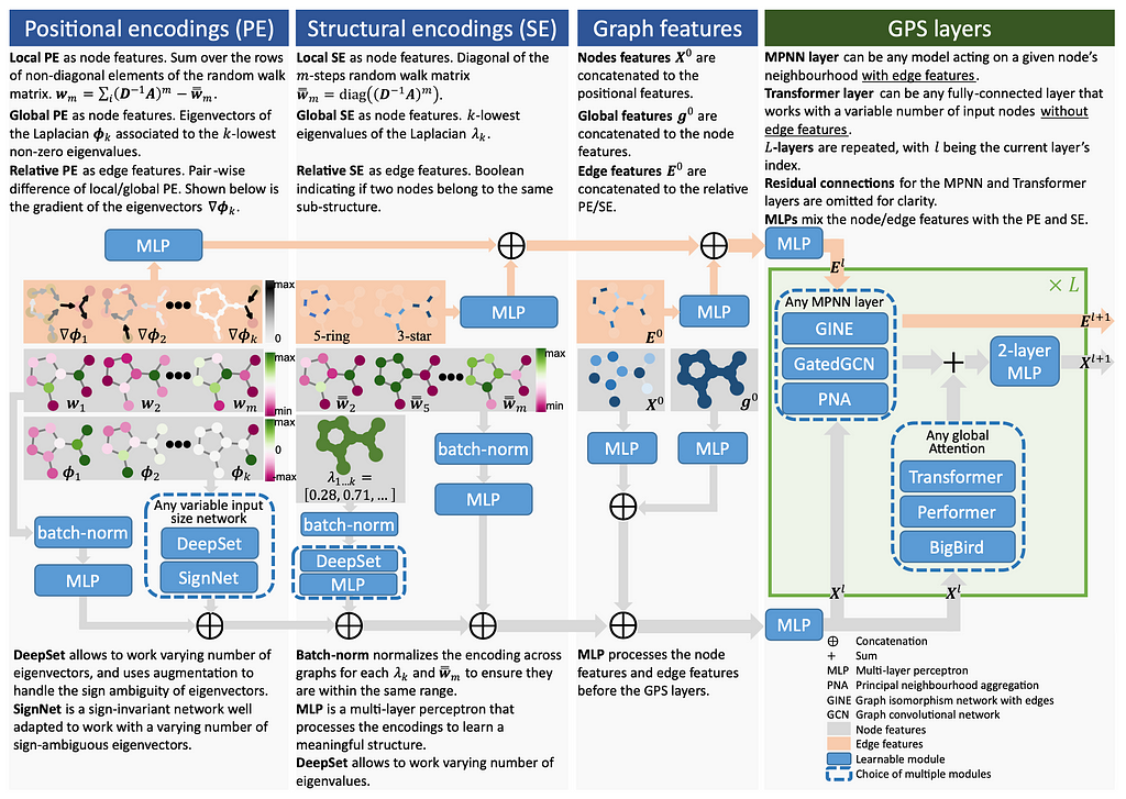
It looks a bit massive, so let’s break it down part by part and check what is happening there.
Overall, the blueprint consists of 3 major components:
- Node identification through positional and structural encodings. After analyzing many recently published methods for adding positionality in graphs, we found they can be broadly grouped into 3 buckets: local, global, and relative. Such features are provably powerful and help to overcome the notorious 1-WL limitation. More on that below!
- Aggregation of node identities with original graph features — those are your input node, edge, and graph features.
- Processing layers (GPS layers) — how we actually process the graphs with constructed features, here combine both local message passing (any MPNNs) and global attention models (any graph transformer)
- (Bonus 🎁) You can combine any positional and structural feature with any processing layer in our new GraphGPS library based on PyTorch-Geometric!
Powerful: Structural and Positional Features
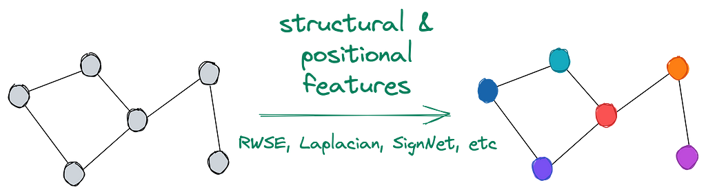
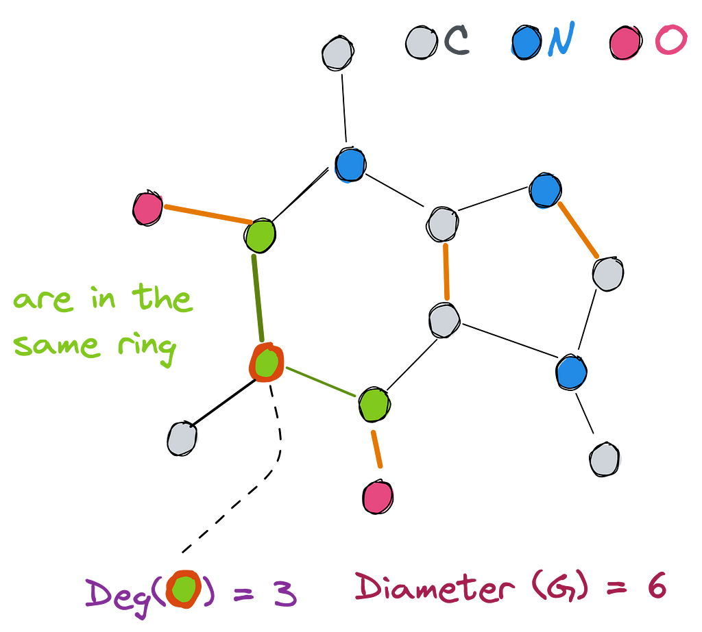
Structural and positional features aim at encoding a unique characteristic of each node or edge. In the most basic case (illustrated below), when all nodes have the same initial features or no features at all, applying positional and structural features helps to distinguish nodes in a graph, assign them with diverse features, and provide at least some sense of graph structure.
We usually separate positional from structural features (although there are works on the theoretical equivalence of those like in Srinivasan & Ribeiro).
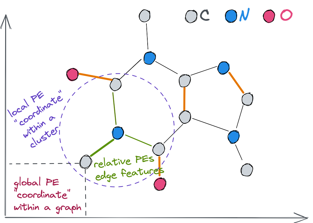
Intuitively, positional features help nodes to answer the question “Where am I?” while structural features answer “What does my neighborhood look like?”
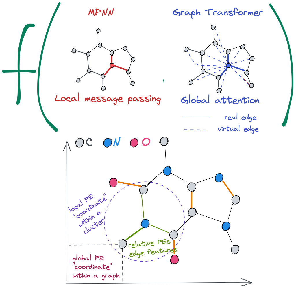
Positional encodings (PEs) provide some notion of the position in space of a given node within a graph. They help a node to answer the question “Where am I?”. Ideally, we’d like to have some sort of Cartesian coordinates for each node, but since graphs are topological structures and there exist an infinite amount of ways to position a graph on a 2D plane, we have to think of something different. Talking about PEs, we categorize existing (and theoretically possible) approaches into 3 branches — local PEs, global PEs, and relative PEs.
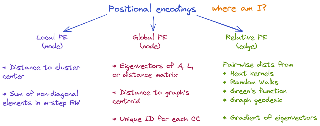
👉 Local PEs (as node features) — within a cluster, the closer two nodes are to each other, the closer their local PE will be, such as the position of a word in a sentence (but not in the text). Examples: (1) distance between a node and the centroid of a cluster containing this node; (2) sum of non-diagonal elements of the random walk matrix of m-steps (m-th power).
👉 Global PEs (as node features) — within a graph, the closer two nodes are, the closer their global PEs are, such as the position of a word in a text. Examples: (1) eigenvectors of the adjacency or Laplacian used in the original Graph Transformer and SAN; (2) distance from the centroid of the whole graph; (3) unique identifier for each connected component
👉 Relative PEs (as edge features) — edge representation that is correlated to the distance given by any local or global PE, such as distance between two worlds. Examples: (1) pair-wise distances obtained from heat kernels, random walks, Green’s function, graph geodesic; (2) gradient of eigenvectors of adjacency or Laplacian, or gradient of any local/global PEs.
Let’s check an example of various PEs on this famous molecule ☕️ (the favorite molecule of Michael Bronstein according to his ICLR’21 keynote).
Structural encodings (SEs) provide a representation of the structure of graphs and subgraphs. They help a node to answer the question “What does my neighborhood look like?”. Similarly, we categorize possible SEs into local, global, and relative, although under a different sauce.
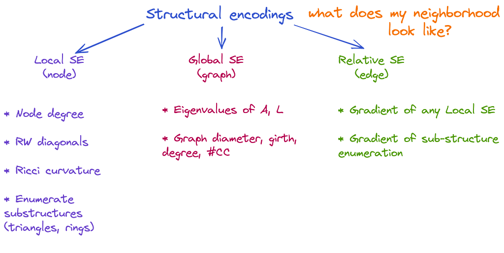
👉 Local SEs (as node features) allow a node to understand what substructures it is a part of. That is, given two nodes and SE of radium m, the more similar are m-hop subgraphs around those nodes, the closer will be their local SEs. Examples: (1) Node degree (used in Graphormer); (2) diagonals of m-steps random walk matrix (RWSE); (3) Ricci curvature; (4) enumerate or count substructures like triangles and rings (Graph Substructure Networks, GNN As Kernel).
👉 Global SEs (as a graph feature) provide the network with information about the global structure of a graph. If we compare two graphs, their global SEs will be close if their structure is similar. Examples: (1) eigenvalues of the adjacency or Laplacian (used in SAN); (2) well-known graph properties like diameter, number of connected components, girth, average degree.
👉 Relative SEs (as edge features) allow two nodes to understand how much their structures differ. Those can be gradients of any local SE or a boolean indicator when two nodes are in the same substructure (eg, as in GSN).
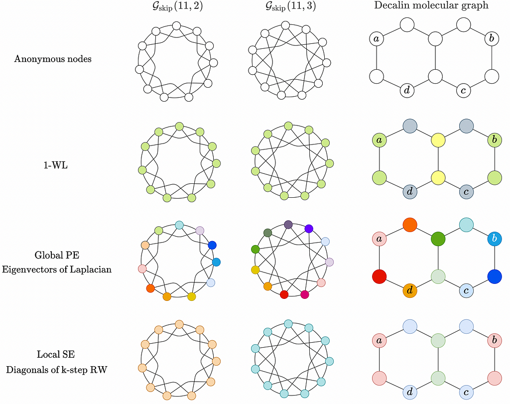
Depending on the graph structure, positional and structural features might bring a lot of expressive power surpassing the 1-WL limit. For instance, in highly-regular Circular Skip Link (CSL) graphs, eigenvectors of Laplacian (Global PEs in our framework) assign unique and different node features for CSL (11, 2) and CSL (11, 3) graphs making them clearly distinguishable (where 1-WL fails).
Aggregation of PEs and SEs
Given that PEs and SEs might be beneficial in different scenarios, why would you limit the model with just one positional / structural feature?
In GraphGPS, we allow to combine any arbitrary amount of PEs and SEs, e.g., 16 Laplacian eigenvectors + eigenvalues + 8d RWSE. In pre-processing, we might have many vectors for each node and we use set aggregation functions that would map them to a single vector to be added to the node feature.
This mechanism enables using subgraph GNNs, SignNets, Equivariant and Stable PEs, k-Subtree SATs, and other models that build node features as complex aggregation functions.
Now, equipped with expressive positional and structural features, we can tackle the final challenge — scalability.
Scalable: Linear Transformers 🚀
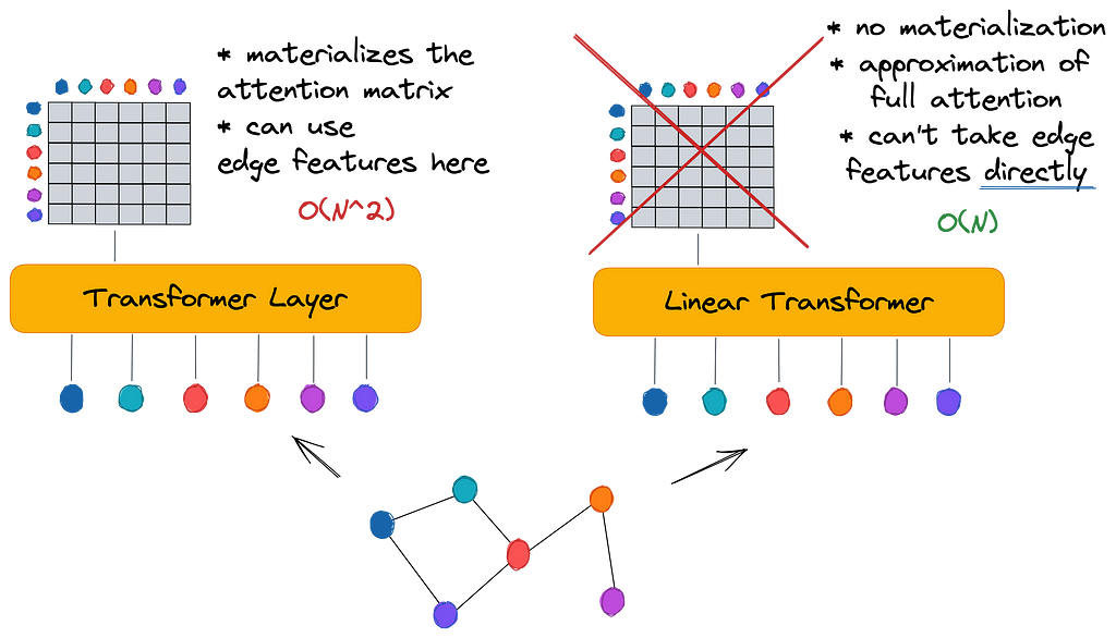
Pretty much all existing graph transformers employ a standard self-attention mechanism materializing the whole N² matrix for a graph of N nodes (thus assuming the graph is fully connected). On one hand, it allows to imbue GTs with edge features (like in Graphormer that used edge features as attention bias) and separate true edges from virtual edges (as in SAN). On the other hand, materializing the attention matrix has square complexity O(N²) making GTs hardly scalable to anything beyond molecular graphs of 50–100 nodes.
Luckily, the vast research around Transformers in NLP recently proposed a number of Linear Transformer architectures such as Linformer, Performer, BigBird to scale attention linearly to the input sequence O(N). The whole Long Range Arena benchmark has been created to evaluate linear transformers on extremely long sequences. The essence of linear transformers is to bypass the computation of the full attention matrix and rather approximate its result with various mathematical “tricks” such as low-rank decomposition in Linformer or softmax kernel approximation in Performer. Generally, this is a very active research area 🔥 and we expect there will be more and more effective approaches coming soon.
Interestingly, there is not much research on linear attention models for graph transformers — to date, we are only aware of the recent ICML 2022 work of Choromanski et al which, unfortunately, did not run experiments on reasonably large graphs.
In GraphGPS, we propose to replace the global attention module (vanilla Transformer) with pretty much any available linear attention module. Applying linear attention leads to two important questions that took us a great deal of experiments to answer:
- Since there is no explicit attention matrix computation, how to incorporate edge features? Do we need edge features in GTs at all?
Answer: Empirically, on the datasets we benchmarked, we found that linear global attention in GraphGPS works well even without edge features (given that edge features are processed by some local message passing GNN). Further, we theoretically demonstrate that linear global attention does not lose edge information when input node features already encode the edge features. - What is the tradeoff between speed and performance of linear attention models?
Answer: The tradeoff is quite beneficial — we did not find major performance drops when switching from square to linear attention models, but found a huge memory improvement. That is, at least in the current benchmarks, you can simply swap the full attention to linear and train models on dramatically larger graphs without huge performance losses. Still, if we want to be more sure about linear global attention performance, there is a need for larger benchmarks with larger graphs and long-range dependencies.
👨🍳 Recipe time — how to get the best out of your GT
Long story short — a tuned GraphGPS, a combination of local and global attention, performs very competitively to more sophisticated and computationally more expensive models and sets a new SOTA on many benchmarks!
For example, in the molecular regression benchmark ZINC, GraphGPS reaches a new all-time low 0.07 MAE. The progress in the field is really fast — last year’s SAN did set a SOTA of 0.139, so we improved the error rate by a solid 50%! 📉
Furthermore, thanks to efficient implementation, we dramatically improved the speed of graph transformers — about 400% faster 🚀 — 196 s/epoch on ogbg-molpcba compared to 883 s/epoch of SAN, the previous SOTA graph transformer model.
We experiment with Performer and BigBird as linear global attention models and scale GraphGPS to graphs of up to 10,000 nodes fitting on a standard 32 GB GPU which is previously unattainable by any graph transformer.
Finally, we open-source the GraphGPS library (akin to the GraphGym environment), where you can easily plug, combine, and configure:
- Any local message passing model with and without edge features
- Any global attention model, eg, full Transformer or any linear architecture
- Any structural (SE) and positional (PE) encoding method
- Any combination of SEs and PEs, eg, Laplacian PEs with Random-Walk RWSE!
- Any method for aggregating SEs and PEs, eg, SignNet or DeepSets
- Run it on any graph dataset supported by PyG or with a custom wrapper
- Run large-scale experiments with Wandb tracking
- And, of course, replicate the results of our experiments
📜 arxiv preprint: https://arxiv.org/abs/2205.12454
🔧 Github repo: https://github.com/rampasek/GraphGPS
GraphGPS: Navigating Graph Transformers was originally published in Towards Data Science on Medium, where people are continuing the conversation by highlighting and responding to this story.
from Towards Data Science - Medium https://ift.tt/TB7WaV9
via RiYo Analytics


No comments