https://ift.tt/qgI6jGf Ref: Pixabay.com Skewed Joins lead to stragglers in a Spark Job bringing down the overall efficiency of the Job. ...

Skewed Joins lead to stragglers in a Spark Job bringing down the overall efficiency of the Job. Here are the five exclusive tips to address Skewed Joins in different situations.
Joins are the one of the most fundamental transformations in a typical data processing routine. A Join operator makes it possible to correlate, enrich and filter across two input datasets. The two input datasets are generally classified as a left dataset and a right dataset based on their placing with respect to the Join clause/operator.
Fundamentally, a Join works on a conditional statement which includes a boolean expression based on the comparison between a left key derived from a record from the left dataset and a right key derived from a record from the right dataset. The left and the right keys are generally called as ‘Join Keys’. The boolean expression is evaluated against each pair of records across the two inputs datasets. Based on boolean output from the evaluation of expression, the conditional statement includes a selection clause to select either one of the record from the pair or a combined record of the records forming the pair.
Performing Joins on Skewed Datasets: A Dataset is considered to be skewed for a Join operation when the distribution of join keys across the records in the dataset is skewed towards a small subset of keys. For example when 80% of records in the datasets contribute to only 20% of Join keys .
Implications of Skewed Datasets for Join: Skewed Datasets, if not handled appropriately, can lead to stragglers in the Join stage (Read this linked story to know more about Stragglers). This brings down the overall execution efficiency of the Spark job. Also, skewed datasets can cause memory overruns on certain executors leading to failure of the Spark job. Therefore, it is important to identify and address Join based stages where large skewed datasets are involved.
Techniques to Address Skewed Joins: Until now you must have seen lot of scattered literature to handle skewed Joins but most of these emphasize 1 or 2 techniques and describe briefly about the details and limitations involved. Considering this scattered description, this particular story is an attempt to provide you with a complete and comprehensive list of five important techniques to handle skewed Joins in every possible scenario:
1) Broadcast Hash Join: In ‘Broadcast Hash’ join, either the left or the right input dataset is broadcasted to the executor. ‘Broadcast Hash’ join is immune to skewed input dataset(s). This is due to the fact that partitioning, in accordance with ‘Join Keys’, is not mandatory on the left and the right dataset. Here, one of the dataset is broadcasted while the other can be appropriately partitioned in suitable manner to achieve uniform parallelism of any scale.
Spark selects ‘Broadcast Hash Join’ based on the Join type and the size of input dataset(s). If the Join type is favorable and the size of dataset to be broadcasted remains below a configurable limit (spark.sql.autoBroadcastJoinThreshold (default 10 MB)), ‘Broadcast Hash Join’ is selected for executing Join. Therefore, if you increase the limit of ‘spark.sql.autoBroadcastJoinThreshold’ to a higher value so that ‘Broadcast Hash Join’ is selected only.
One can also use broadcast hints in the SQL queries on either of the input datasets based on the Join type to force Spark to use ‘Broadcast Hash Join’ irrespective of ‘spark.sql.autoBroadcastJoinThreshold’ value.
Therefore, if one could afford memory for the executors, ‘Broadcast Hash’ join should be adopted for faster execution of skewed join. However here are some salient points that needs to be considered while planning to use this fastest method:
- Not Applicable for Full Outer Join.
- For Inner Join, executor memory should accommodate at least smaller of the two input dataset.
- For Left , Left Anti and Left Semi Joins, executor memory should accommodate the right input dataset as the right one needs to be broadcasted.
- For Right , Right Anti and Right Semi Joins, executor memory should accommodate the left input dataset as the left one needs to be broadcasted.
- There is also a considerable demand of execution memory on executors based on the size of broadcasted dataset.
2) Iterative Broadcast Join: ‘Iterative Broadcast’ technique is an adaption of ‘Broadcast Hash’ join in order to handle larger skewed datasets. It is useful in situations where either of the input dataset cannot be broadcasted to executors. This may happen due to the constraints on the executor memory limits.
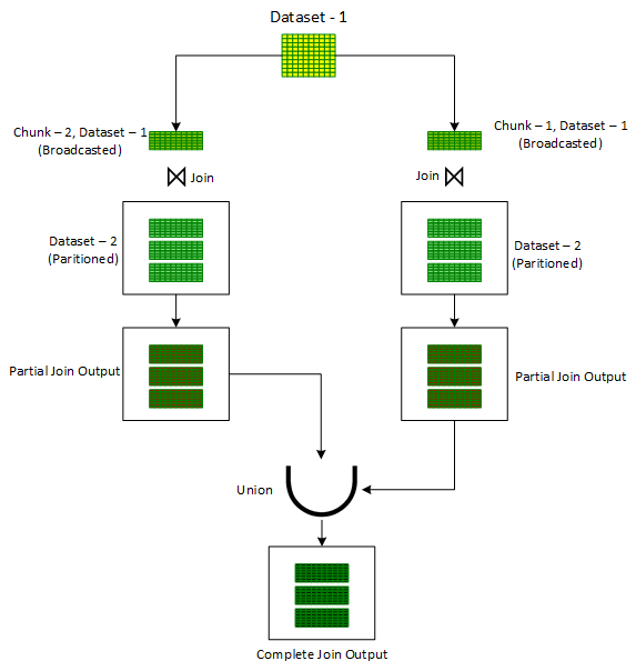
In order to deal with such scenarios, ‘Iterative Broadcast’ technique breaks downs one of the input data set (preferably the smaller one) into one or more smaller chunks thereby ensuring that each of the resulting chunk can be easily broadcasted. These smaller chunks are then joined one by one with the other unbroken input dataset using the standard ‘Broadcast Hash’ Join. Outputs from these multiple joins is finally combined together using the ‘Union’ operator to produce the final output.
One of the ways in which a Dataset can be broken into smaller chunks is to assign a random number out of the desired number of chunks to each record of the Dataset in a newly added column, ‘chunkId’. Once this new column is ready, a for loop is initiated to iterate on chunk numbers. For each iteration , firstly the records are filtered on the ‘chunkId’ column corresponding to current iteration chunk number. The filtered dataset, in each iteration, is then joined with the unbroken other input dataset using the standard ‘Broadcast Hash’ Join to get the partial joined output. The partial joined output is then combined with the previous partial joined output. After the loop is exited, one would get the overall output of the join operation of the two original datasets. This technique is shown below in Figure 1.

However, in contrast to ‘Broadcast Hash Join’, ‘Iterative Broadcast Join’ is limited to ‘Inner Joins’ only. It cannot handle Full Outer Joins, Left Joins and Right Joins. However, for ‘Inner Joins’, it can handle skewness on both the datasets.
3) Salted Sort Merge Join: ‘Sort Merge’ approach is very robust in handling Joins in case of resource constraints. Extending the same, the salted version of ‘Sort Merge ’ can be used very effectively when one wants to join a large skewed dataset with a smaller non-skewed dataset but there are constraints on the executor’s memory.
Additionally, the Salted Sort Merge version can also be used to perform Left Join of smaller non-skewed dataset with the larger skewed dataset which is not possible with Broadcast Hash Join even when the smaller dataset can be broadcasted to executors. However, to make sure that Sort Merge Join is selected by the Spark, one has to turn off the ‘Broadcast Hash Join’ approach. This can be done by setting ‘spark.sql.autoBroadcastJoinThreshold’ to -1.
The working of ‘Salted Sort Merge’ Join is kind of similar to ‘Iterative Broadcast Hash’ Join. An additional column ‘salt key’ is introduced in one of the skewed input dataset. After this, for every record, a number is randomly assigned from a selected range of salt key values for the ‘salt key’ column.
After salting the skewed input dataset, a loop is initiated on salt key values in the selected range. For every salt key value being iterated in the loop, the salted input dataset is first filtered for the iterated salt key value, after filtration, the salted filtered input dataset is joined together with the other unsalted input dataset to produce a partial joined output. To produce the final joined output, all the partial joined outputs are combined together using the Union operator.
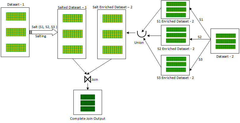
An alternative approach also exists for ‘Salted Sort Merge’ approach. In this, for every salt key value being iterated in the loop, the second non skewed input dataset is enriched with the current iterated salt key value by repeating the the same value in the new ‘salt’ column to produce a partial salt enriched dataset. All these partial enriched datasets are combined using the ‘Union’ operator to produce a combined salt enriched dataset version of the second non-skewed dataset. After this, the first skewed salted dataset is Joined with the second salt enriched dataset to produce the final joined output. This approach is shown below in the Figure 3:

A yet other alternative approach also exists for ‘Salted Sort Merge’ approach. In this approach, after salting the skewed input dataset with the additional ‘salt key’ column, a ‘salt’ column is also introduced in the unsalted non-skewed dataset. The ‘salt’ column contains a fixed value (across all records) equal to an array made up of all values of salt keys in the earlier selected range. Afterwards, this dataset is then exploded on the ‘salt’ column. The exploded dataset is then joined with the earlier salted skewed input dataset with an additional join condition on the equality of ‘salt’ and ‘salt key’ to produce the final joined output.
Salted Sort Merge Join cannot handle Full Outer Join. Also, it cannot handle skewness on both the input dataset. It can handle skew only in the left dataset in the Left Joins category (Outer, Semi and Anti). Similarly, it can handle skew only in the right dataset in the Right Joins category.
4) AQE (Advanced Query Execution): AQE is a suite of runtime optimization features which is now enabled by default from Spark 3.0. One of the key feature this suite packs is the capability to automatically optimize Joins for skewed Datasets.
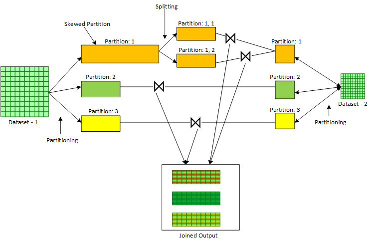
AQE performs this optimization generally for ‘Sort Merge Joins’ of a skewed dataset with a non- skewed dataset. AQE operates at partitioning step of a Sort Merge Join where the two input Datasets are firstly partitioned based on corresponding Join Key. After the shuffle blocks are written by the MapTasks during partitioning, Spark Execution Engine gets stats on the size of each shuffled partitions. With these stats available from Spark Execution Engine, AQE can determine, in tandem with certain configurable parameters, if certain partitions are skewed or not. In case certain partitions are found as skewed, AQE breaks down these partitions into smaller partitions. This breakdown is controller by a set of configurable parameters. The smaller partitions resulting from the breakdown of a bigger skewed partition are then joined with a copy of corresponding partition of the other non skewed input dataset. The process is shown below in Figure 3.

Following are the config parameters that affect skewed join optimization feature in AQE:
“spark.sql.adaptive.skewJoin.enabled” : This boolean parameter controls whether skewed join optimization is turned on or off. Default value is true.
“spark.sql.adaptive.skewJoin.skewedPartitionFactor”: This integer parameter controls the interpretation of a skewed partition. Default value is 5.
“spark.sql.adaptive.skewJoin.skewedPartitionThresholdInBytes”: This parameter in MBs also controls the interpretation of a skewed partition. Default value is 256 MB.
A partition is considered skewed when both (partition size > skewedPartitionFactor * median partition size) and (partition size > skewedPartitionThresholdInBytes) are true.
AQE like ‘Broadcast Hash Join’ and ‘Salted Sort Merge Join’ cannot handle ‘Full Outer Join’. Also, it cannot handle skewedness on both the input dataset. Therefore, as in case of ‘Salted Sorted Merge Join’, AQE can handle skew only in the left dataset in the Left Joins category (Outer, Semi and Anti) and skew in the right dataset in the Right Joins category.
5) Broadcast MapPartitions Join: ‘Broadcast MapPartitions Join’ is the only mechanism to fasten a skewed ‘Full Outer Join’ between a large skewed dataset and a smaller non-skewed dataset. In this approach, the smaller of the two input dataset is broadcasted to executors while the Join logic is manually provisioned in the ‘MapPartitions’ transformation which is invoked on the larger non-broadcasted dataset.
Although ‘Broadcast MapPartitions Join’ supports all type of Joins and can handle skew in either or both of the dataset, the only limitation is that it requires considerable memory on executors. The larger executor memory is required to broadcast one of the smaller input dataset, and to support intermediate in-memory collection for manual Join provision.
I hope the above blog has given you a good perspective of handling skewed Joins in your Spark applications. With this background, I would encourage you all to explore one of these options whenever you encounter stragglers or memory overruns in Join stages of the your Spark applications.
In case you would like to have code snippets related to each of these technique, you could reach out to me @ LinkedIn.
Five Tips to Fasten Skewed Joins in Apache Spark was originally published in Towards Data Science on Medium, where people are continuing the conversation by highlighting and responding to this story.
from Towards Data Science - Medium https://ift.tt/YkQEgU4
via RiYo Analytics

No comments