https://ift.tt/98QWMCU Stochastic Processes Simulation — Geometric Brownian Motion Part 4 of the Stochastic Processes Simulation series. S...
Stochastic Processes Simulation — Geometric Brownian Motion
Part 4 of the Stochastic Processes Simulation series. Simulating geometric Brownian motion in Python from scratch.
Geometric Brownian motion is perhaps the most famous stochastic process aside from Brownian motion itself. It arises when we consider a process whose increments’ variance is proportional to the value of the process.
In this story, we will discuss geometric (exponential) Brownian motion. We will learn how to simulate such a process and estimate the necessary parameters, for a simulation, from data. Our concrete goal will be to simulate many, possibly correlated, geometric Brownian motions.
I’ve chosen to use many elements from the object-oriented paradigm mainly because this story will pave the way for the next story, about generalized Brownian motion, in the series. This way, we will be able to extend the code without rewriting it.
We will use the code developed in the first story, about Brownian motion, of the Stochastic Processes Simulation series throughout this story. So if you haven’t checked it out, do it first.
Table of contents
- The equation for the process
- Code structure and architecture
- Constant processes
- Drift process
- Sigma process
- Initial values
- The simulation, putting the pieces together
- Estimate constant parameters from data
- Estimate correlation from data
- Simulation from data
- Code summary
- Final words
The equation for the process
The SDE (stochastic differential equation) for the process is:

where W_t is a Brownian motion. In other words, the quotient of the differential and the process itself follows a diffusive process (Itô process).
Using elementary stochastic calculus (check the references for details) we can easily integrate the SDE in closed-form:

This equation considers the possibility that μ and σ are functions of t and W, this is why this equation is known as generalized geometric Brownian motion.
When μ and σ are constant then the equation is much simpler:

This is the famous geometric Brownian Motion.
Code structure and architecture
A priori, we may not know the form of μ and σ. Ok, you got me here; this story is about geometric Brownian motion, so μ and σ should be constant.
But what happens if they are not? What happens if μ and σ could be deterministic functions of time or other stochastic processes?
If we were to code this in a naive function, we would need arguments (two of them) to select the option for μ and σ. Such an approach would make the internal structure of the function very messy, with many cases considered there (suppose there are m choices for building μ and σ, the number of cases would then be m x n). Furthermore, if we were to introduce another function for either μ or σ, we would need to change said function — a recipe for disaster.
We won’t do this. Instead, we will walk down the OO (object-oriented design) path and establish interfaces (abstract) for what μ and σ objects should be. Then we create a generalized Brownian motion object which depends on these abstract interfaces instead of concrete implementations. This way, we would not need to change the generalized Brownian motion object whenever we change μ or σ objects.
At first, this OO approach may seem longer; but remember, the shortest path seems longer. In the end, it will be worth it.
Remember, our goal is to generate many Brownian motions; hence, our interfaces should be able to create many processes simultaneously.
Constant processes
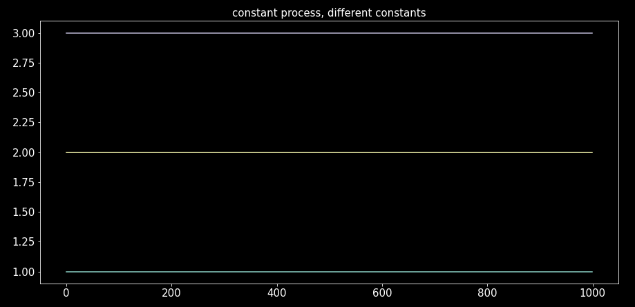
As I mentioned in the previous section, this story is about geometric Brownian motion; hence, μ and σ are constant. However, achieve the generality we seek through our OO approach. They should be constant processes rather than simple constant numbers. We will create a small object to generate constant processes (a 2D array with T rows where each column is constant). The peculiarity of this array is that the argument which defines the actual constants (“constants”) can be:
- A float, in which case all processes have the same constant, and we need the argument “n_procs” to define the number of processes (columns).
- A tuple of floats, in which case each process has a different constant defined by the tuple. The “n_procs” argument is ignored. The resulting array’s columns are indexed in the same order as the constant tuple.
Let’s take the “ConstantProcs” class for a spin:
and plot the constant processes (not much fun, just straight lines, but we need to perform the sanity check):
Drift process
Here is our first example of the OO interfaces. The following protocol is the interface for the drift process:
The drift process, in this case, is constant. So we wrap our “ConstantProcs” object inside the following class, which implements the “Drift” protocol. We inherit from “ConstantProcs” to make the wrapping more explicit and avoid duplicated code.
Sigma process
This is the interface for the sigma process:
Which, again, is constant. Utterly analogous to the previous section, we wrap “ConstantProcs” inside a class that complies with the “Sigma” protocol.
Initial values
Initial values are the values for P_0 as they appear in the geometric Brownian motion equation from the first section of the story. Here is another example where we need an abstract interface (protocol). The strategy for choosing the initial values might change according to our needs. However, this should not change the generalized Brownian motion object. In this case, the protocol does not require a 2D array but rather a 1D array where each vector value corresponds to the initial value (P_0) for each process.
The first behavior that comes to mind is a random choice. We want to input an interval of values and then get random values uniformly sampled. So we do just that. We implement such logic, making it compliant with the “InitP” protocol:
Another behavior we want is to get P_0s from data. If we input a matrix (2D array with processes indexed as columns), the initial values are taken from it. Either the first values or the last values are used as P_0. So we code that.
We can see here that we can build any object we want, and as long it is compliant with the protocol, it will work with no ripples of code rewriting.
As an example, we make an instance of the random init values object:
The simulation, putting the pieces together
At last, we come to coding the geometric Brownian motion, and you guessed it correctly, we will build a class for it. This class will depend on abstractions for μ (Drift protocol), σ (Sigma protocol), and P_0 (InitP protocol). It will also depend on ρ, the correlation coefficient for the processes.
The following code makes use of the “brownian_motion” library, coded in the first story of the series. Save that code under the name “brownian_motion.py” and place it in the directory where you intend to run the code.
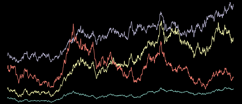
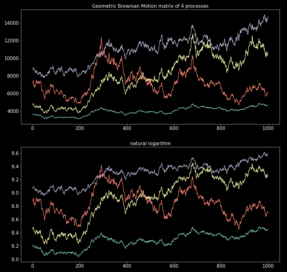
This is an example of how we build the objects for μ, σ, and P_0 and then inject them to “GenGeoBrownian”:
plot the processes in the columns of “P_mat”:
Estimate constant parameters from data
We’ve simulated geometric Brownian processes, and now it is time to estimate μ and σ from data.
We know that the diffusion increments are normally distributed with mean μ and variance σ². Using the Euler-Maruyama method for discrete approximation (forward differences for the stochastic differentials) and making Δt = 1:

Using this equation, we can estimate μ and σ by taking the mean and standard deviation of ΔP_t /P_t, respectively.
We estimate tuples of constants from a matrix of processes (“proc_mat”), as the input for “ConstantDrift” and “ConstantSigma” objects is a tuple:
An example of how to use these functions:
Estimate correlation from data
To estimate the correlation, we require for the simulation (a single ρ number) we calculate the correlation matrix (pairwise correlation) for the diffusion increments and then take the average of all the entries excluding the diagonal (which invariably contains 1s).
Simulation from data
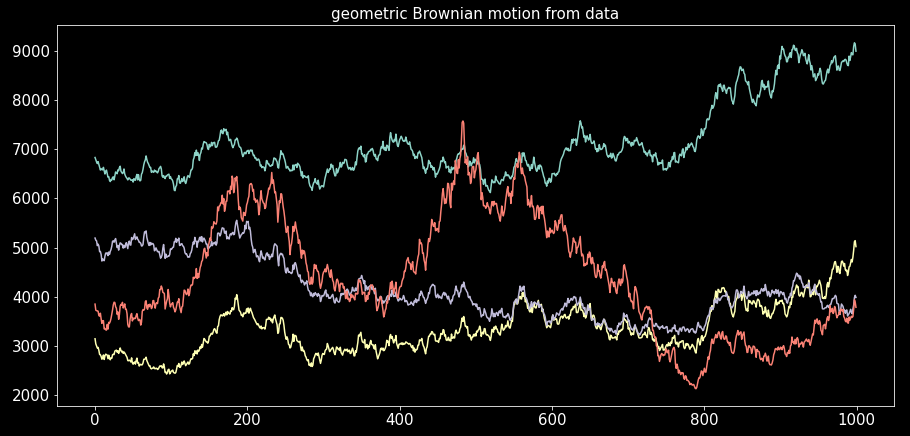
Finally, an example of usage for the tools we’ve just developed in a real example. So far, we’ve used only NumPy arrays throughout the code. In practice, we probably would get the processes’ data in a pandas DataFrame. The following snippet shows how to perform the necessary estimations and create the object instances:
Once the “GenGeoBrownian” instance has been created, generating processes is very simple:
plotting:
Code Summary
There was quite a lot of code in this story, albeit mainly due to my extensive docstrings. Some of the criticisms of OO is that it is too verbose; it is, but in this case, it has given us the flexibility we require.
Here is the code summary of all the tools coded in the story:
Final words
After all the hard work, we successfully simulated many correlated geometric Brownian motions and estimated the necessary parameters from data for such simulations. We also created the interfaces for more complex processes for μ and σ. The interface OO approach will pay off in the next story of the series, where we will discuss generalized Brownian motion.
References
[1] B. Øksendal, Stochastic Differential Equations (2013), Sixth Edition, Springer.
Follow me on Medium and subscribe to get the updates on the next stories as soon as they come out.
I hope this story was useful for you. If I missed anything, please let me know.
Navigate through the Stochastic Processes Simulation series
Previous stories in the series:
- Stochastic Processes Simulation — Brownian Motion, The Basics
- Stochastic Processes Simulation — The Ornstein Uhlenbeck Process
- Stochastic Processes Simulation — The Cox-Ingersoll-Ross Process
Stochastic Processes Simulation — Geometric Brownian Motion was originally published in Towards Data Science on Medium, where people are continuing the conversation by highlighting and responding to this story.
from Towards Data Science - Medium https://ift.tt/SwhquT8
via RiYo Analytics


No comments