https://ift.tt/Vv89bzA Regularizing, Bagging, Stacking, and More Image by author Time series data typically has four components: Auto...
Regularizing, Bagging, Stacking, and More
Time series data typically has four components:
- Autoregression
- Seasonality
- Trend
- Residual
Predict these components, and you can forecast almost any time series. Sounds easy enough, right?
Well, not exactly. There is a lot of ambiguity around the best ways to specify a model so that it can account for these elements correctly, and much research in the past years has been released to find the best ways to do so, with state-of-the art models, such as recurrent and other neural network models, taking center stage. Furthermore, many series have other effects that should be accounted for, such as holidays and structural breaks.
All this to say, predicting any given series is often not as easy as using a linear regression. Non-linear estimators and ensemble methods can be combined with linear methods to find the best approach for any series. In this post, I overview a sample of these models from the Scitkit-learn library and how they can be utilized to maximize accuracy. These methods are applied on the Daily Visitors Dataset with a little over 2,000 observations that can be found on Kaggle or RegressIt. Special thanks to Professor Bob Nau for supplying it!
The structure of this blog post is fairly repetitive, with the same graphs and evaluation metrics examined for each applied model. If you are already familiar with Scikit-learn models and APIs like MLR, XGBoost, and others, you can skip to the Bagging and Stacking sections to overview something that might be a little different. You can find the full notebook on GitHub.
Prepare Models
All models are run using the scalecast package, which contains results and wraps Scikit-learn and other models around time-series data. All its forecasting uses a dynamic multi-step forecast by default, which returns more reasonable accuracy/error metrics over the whole forecast horizon than an average of one-step forecasts would.
pip install scalecast
Give the package a star on GitHub if you find it interesting.
We will use a forecast horizon of 60 days and also use a 60-day set to validate each model and tune its hyperparameters. All models will be tested on 20% of the original data:
f=Forecaster(y=data['First.Time.Visits'],current_dates=data['Date'])
f.generate_future_dates(60)
f.set_test_length(.2)
f.set_validation_length(60)
From EDA (not shown here), it appears that there is autocorrelation up to 4 weeks in the past, and that the first 7 dependent-variable lags could be significant.
f.add_ar_terms(7) # 7 auto-regressive terms
f.add_AR_terms((4,7)) # 4 seasonal terms spaced 7 apart
For this dataset, there are several seasonal elements which must be accounted for, including daily, weekly, monthly, and quarterly fluctuations.
f.add_seasonal_regressors(
    'month',
    'quarter',
    'week',
    'dayofyear',
    raw=False,
    sincos=True
) # fourier transformation
f.add_seasonal_regressors(
    'dayofweek',
    'is_leap_year',
    'week',
    raw=False,
    dummy=True,
    drop_first=True
) # dummy vars
Finally, we can model the series’ trend by adding the year variable:
f.add_seasonal_regressors('year')
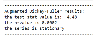
For all these models, you typically want to feed them stationary time series data. We can confirm this data is stationary with the Augmented Dickey-Fuller test:
MLR
We will start simple and try applying Multiple Linear Regression (MLR). This model is fast, simple, and has no hyperparameters to tune. It often obtains great accuracy and can be hard to beat even with more advanced methods.
It assumes all components in the model can be combined in a linear manner to predict the final output:

Where j is the number of added regressors (in our case, the AR, seasonal, and trend components) and alpha the corresponding coefficient. In our code, calling this function looks like:
f.set_estimator('mlr')
f.manual_forecast()
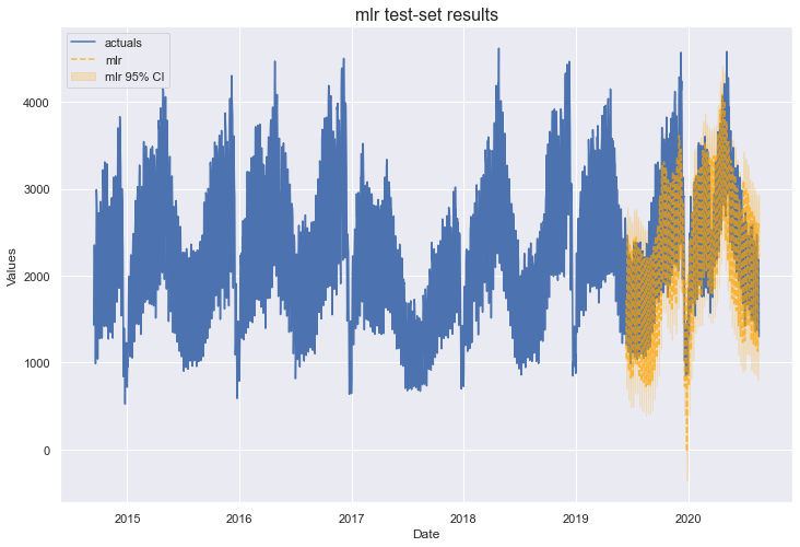

It’s worth noting that a more common application of a linear method for time series is ARIMA, which also uses the series’ errors as a regressor. MLR assumes that the series’ errors are uncorrelated, which is spurious in time series. That being said, in our analysis, a test-set Mean Absolute Percentage Error of 13% and R2 of 76% are obtained with MLR. Let’s see if that can be beat by adding complexity.
Lasso
The next three models reviewed, Lasso, Ridge and ElasticNet, all use the same underlying function of the MLR to make predictions, but the way the coefficients are estimated is different. There are L1 and L2 regularization parameters, which serve to lessen the coefficients’ magnitudes, which in turn reduces overfitting and can lead to better out-of-sample predictions. This can be a good technique to try in our case since the MLR’s in-sample R2 score is 95%, significantly larger than the out-of-sample R2 of 76%, indicating overfitting.
There is one parameter to estimate with lasso — the size of the L1 penalty parameter, or alpha. We can do this via a grid-search of 100 alpha values on the validation set of data. It looks like this:
f.add_sklearn_estimator(Lasso,'lasso')
f.set_estimator('lasso')
lasso_grid = {'alpha':np.linspace(0,2,100)}
f.ingest_grid(lasso_grid)
f.tune()
f.auto_forecast()
It is important that Lasso (as well as Ridge and ElasticNet) uses scaled inputs so that the penalty parameter is balanced to all coefficients. Scalecast uses a MinMax scaler by default.
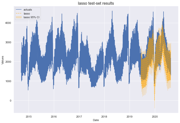

The optimal alpha value selected was 0.081. This model neither improved the out-of-sample accuracy from the MLR model, nor reduced overfitting. We can try again with the Ridge model.
Ridge
Ridge is similar to Lasso, except it uses an L2 penalty. The difference here is that an L1 penalty can reduce certain coefficients to zero, whereas Ridge can reduce coefficients to near-zero only. Usually, both models produce similar results. We can tune the Ridge model with the same grid we created for the Lasso model.
f.set_estimator('ridge')
f.ingest_grid(lasso_grid)
f.tune()
f.auto_forecast()
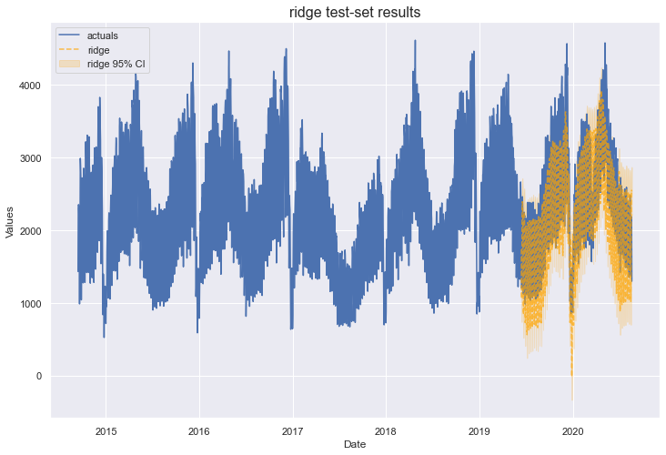

The optimal alpha selected for the Ridge model was 0.384 and its results were similar to, if not a little worse than, the lasso model. We have one more model that can apply regularization to MLR: ElasticNet.
ElasticNet
The ElasticNet model offered by Scikit-learn will predict outputs using a linear model, but now it will mix L1 and L2 penalties. The key parameters to tune now are:
- The L1/L2 penalty ratio (l1_ratio )
- The penalty value (alpha )
Scalecast offers a good default validation grid for ElasticNet, so we don’t have to create one.
f.set_estimator('elasticnet')
f.tune()
f.auto_forecast()
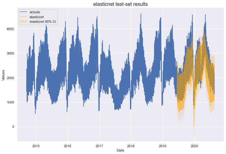

The optimal parameters for ElasticNet were an l1_ratio of 1, which makes it equivalent to a lasso model, and an alpha of 0.3. It performed about as well as the Lasso and Ridge models and again, did not reduce overfitting.
Random Forest
Having exhausted several linear methods to estimate this series, we can move to non-linear methods. One of the most popular of these is Random Forest, a tree-based ensemble method. It functions by aggregating several tree estimators with bootstrapped samples (sampling with replacement) of the original dataset. Each sample can utilize different rows and columns of the original dataset and the final results are an average of a specified number of underlying decision-tree estimators applied on each sample.
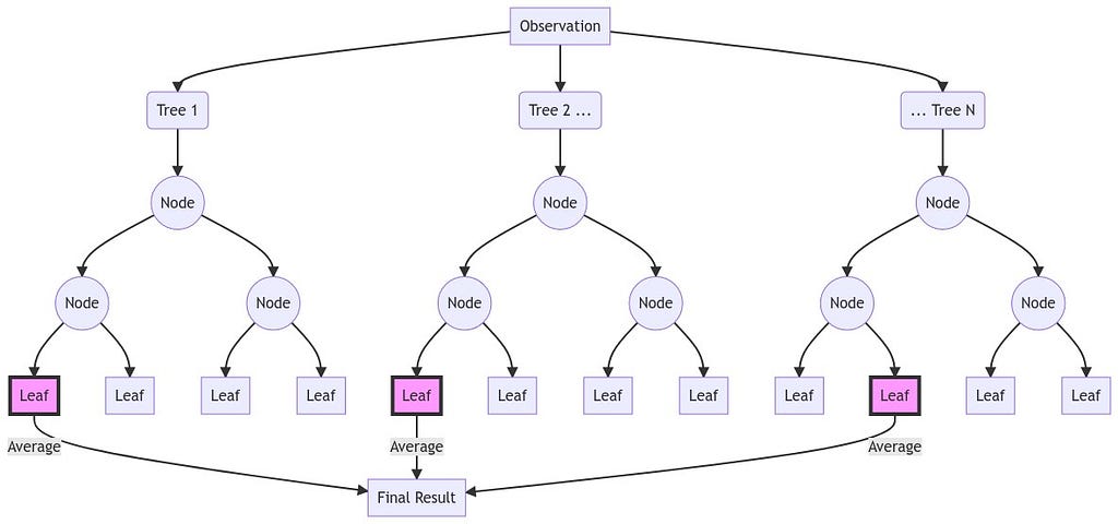
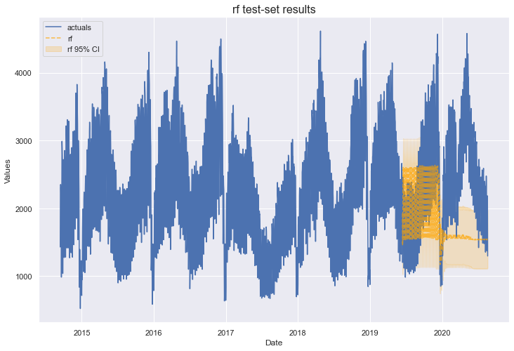
Several criticisms of using Random Forest for time series forecasting are raised from time-to-time, such as estimated values not able to be greater than the largest observed value or less than the smallest observed value. Sometimes, this problem can be circumvented by ensuring stationary data only is fed to the estimator. But generally, this model is not known for its time series prowess. Let’s see how it does in this example. We can specify our own validation grid.
rf_grid = {
     'max_depth':[2,3,4,5],
     'n_estimators':[100,200,500],
     'max_features':['auto','sqrt','log2'],
     'max_samples':[.75,.9,1],
}
And then run the forecast.
f.set_estimator('rf')
f.ingest_grid(rf_grid)
f.tune()
f.auto_forecast()
From here on, I have to paste two tables for model benchmarking or else it becomes impossible to read. The bottom table’s rows correspond with the models listed in the top table.

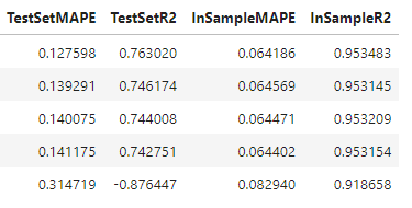
Unfortunately, we didn’t have much luck with Random Forest. It performed significantly worse than the ones evaluated before it. However, the concept of bootstrapped sampling introduced here will be integral once we overview forecasting with the BaggingRegressor model.
XGBoost
XGBoost is a difficult model to briefly explain, so I defer to the articles here (for beginners) and here (for a deep dive) to do so, if the reader is interested. The basic idea is that similar to Random Forest, estimations are made through a series of decision trees, where final results are a type of weighted average of each underlying estimation. Unlike Random Forest, trees are built sequentially, where each subsequent tree models the residuals of the tree that came before it, hoping to minimize the final residuals as much as possible. Sampling is not random but rather, based on the weaknesses of the previous tree. In this way, results are obtained by boosting the samples, whereas Random Forest uses bootstrapped aggregation where each tree and sample are independent of the others. This is an oversimplification of what’s really happening underneath the hood, so please read the linked articles if this explanation did not satisfy you. There are many hyperparameters to tune in such a model and we can build a grid like this:
xgboost_grid = {
     'n_estimators':[150,200,250],
     'scale_pos_weight':[5,10],
     'learning_rate':[0.1,0.2],
     'gamma':[0,3,5],
     'subsample':[0.8,0.9]
}
Evaluating the model:
f.set_estimator('xgboost')
f.ingest_grid(xgboost_grid)
f.tune()
f.auto_forecast()
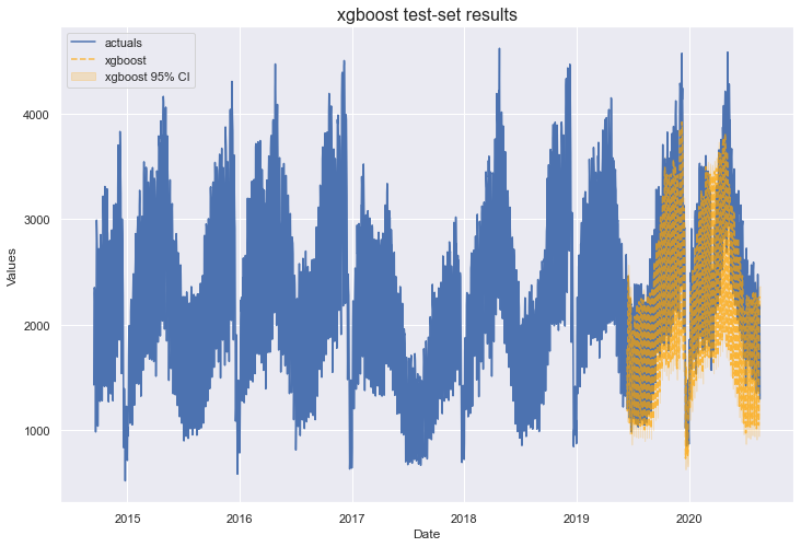

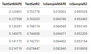
XGBoost out-performed MLR with a test-set MAPE of 12%. However, it appears even more overfit, with an in-sample R2 score close to 100%.
By now, hopefully you get the idea of how these models were built and evaluated. In the provided notebook, you can also see examples for LightGBM (Microsoft’s boosted tree model that is similar to XGBoost), Stochastic Gradient Descent, and K-nearest Neighbors. For the sake of brevity, I will skip to the Bagging and Stacking models to finish out the post.
Bagging
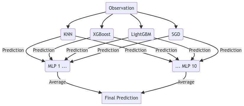
The BaggingRegressor from Scikit-learn uses the same sampling concept introduced in the Random Forest section of this post, but instead of each underlying estimator being a decision tree, we can use any model we’d like. In this case, I specified 10 Multi-Level Perceptron neural network models with three layers of 100 units each and the LBFGS solver. Each data subset is allowed to use 90% of the original dataset’s size to sample observations and also uses 50% of the original dataset’s features at random. In the code, it looks like this:
f.add_sklearn_estimator(BaggingRegressor,'bagging')
f.set_estimator('bagging')
f.manual_forecast(
     base_estimator = MLPRegressor(
         hidden_layer_sizes=(100,100,100),
         solver='lbfgs'
     ),
     max_samples = 0.9,
     max_features = 0.5,
)
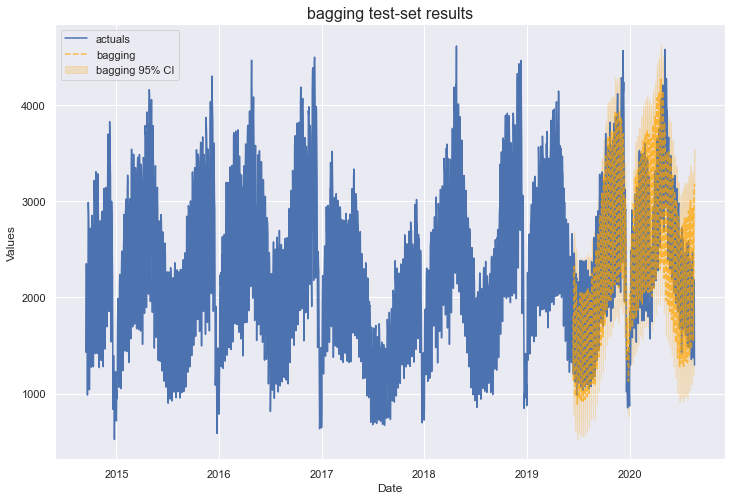
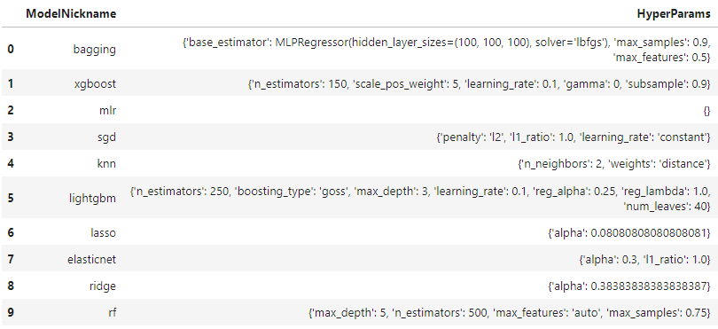
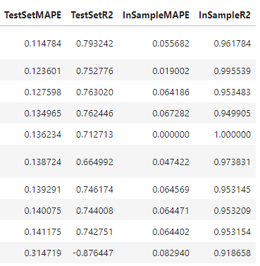
This model has performed the best so far with a test-set MAPE of 11% and test-set R2 score of 79%. This is pretty significantly better than the next best models by the same metrics, XGBoost and MLR.
Stacking
The last model overviewed is the StackingRegressor. It creates a new estimator that uses the predictions from other specified models to create a final prediction. It makes this final prediction with an estimator passed to the final_estimator parameter.
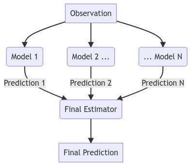
In our case, we are stacking four of the models that evaluated the best out-of-sample on this dataset:
- K-nearest Neighbors (KNN)
- XGBoost
- LightGBM
- Stochastic Gradient Descent (SGD)
The final estimator is the bagging estimator we defined in the previous section.

The advantage to using the BaggingRegressor as the final estimator is that even though the KNN and XGBoost models were highly overfit and the MLP models should conceptually weight their predictions artificially high accordingly, because this model is trained with only half of the features input to any given MLP model, it should also learn to trust the predictions from the two models that were not as overfit: LightGBM and SGD. The model is therefore evaluated as such:
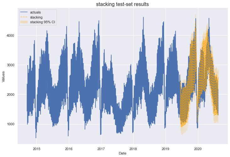
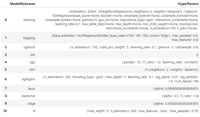
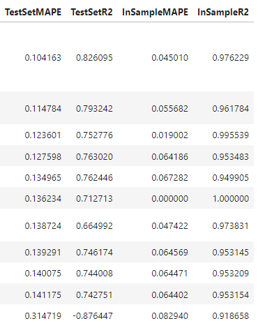
It’s not always the case that adding complexity to models will improve results, but that appears to be what’s happening here. Our stacking model clearly outperformed the others, with a test-set MAPE of 10% and test-set R2 score of 83%. It also has in-sample metrics comparable to the evaluated MLR.
Backtesting
To further validate our models, we can back-test them. This is a process of iteratively evaluating their accuracy over the last n-many forecast horizons to see what results would have actually been achieved had that model been implemented, trained only on the observations that come before each forecast horizon. By default, scalecast selects 10 forecast horizons with a length determined by the number of future dates generated in the object (in our case, 60). Here’s what it looks like in code:
f.backtest('stacking')
f.export_backtest_metrics('stacking')

This tells us that on average, using a forecast length of 60 days, our model would have obtained a MAPE score of 7% and R2 of 76%. This is a good way to validate that the model didn’t just get lucky with the particular test-set fed to it and can actually generalize to unseen data.
Conclusion
This post introduced several modeling concepts for forecasting, including linear methods (MLR, Lasso, Ridge), Tree ensembles (Random Forest, XGBoost, LightGBM), bagging, and stacking. By ramping up the complexity of the non-linear methods applied to it and using clever sampling methods, we obtained a test-set MAPE score of 10% on a test-set with about 400 observations. I hope this example was able to spark some ideas of your own and I appreciate you following along! If you found this overview helpful, give the scalecast package a star on GitHub.
Expand your Time Series Arsenal with These Models was originally published in Towards Data Science on Medium, where people are continuing the conversation by highlighting and responding to this story.
from Towards Data Science - Medium https://ift.tt/zbKJyOn
via RiYo Analytics

No comments