https://ift.tt/YstWnJx Never mind the maneuvers; minimize the Dickey-Fuller statistic directly to achieve a stationary time series. Full Py...
Never mind the maneuvers; minimize the Dickey-Fuller statistic directly to achieve a stationary time series. Full Python code.
There are many methods for finding cointegrating vectors. Some methods leverage OLS, others matrix eigendecomposition. Regardless of the method, it is customary to do a sanity check by performing a stationarity test on the resulting time series.
The workflow goes something like this:
- find the cointegrating vector (the method of your choice)
- do a stationarity test on the time series generated with the vector of step 1 and discard spurious results
Enter the Dickey-Fuller test. More often than not, the stationarity test we will use in step 2 is precisely the Dickey-Fuller test statistic.
If we end up checking if the Dickey-Fuller statistic is small enough to state whether our cointegration method was successful, why not simply minimize the Dickey-Fuller statistic in the first place?
This story will tackle the cointegration problem by directly minimizing the Dickey-Fuller test statistic. Usually, I would think twice before using plain function optimization as the main driver of an algorithm. Sure, we could throw any function to an optimizer from the many libraries available in Python and see what happens. I’ve done that many times before. It is generally not a very good idea.
Many things can go wrong with function optimization, especially when the function is relatively unknown; among them:
- function calls could be expensive
- the function could be noisy
- the function could be non-convex
Even if the optimization works well, it could be dead slow.
In this story, we will address all these issues. We will code a method comparable in speed to the Johansen method and BTCD and with the same or even more reliability. However, there will be some math involved, so be warned. To successfully optimize the function (and not take forever), we will calculate the gradient and the Hessian matrix for the Dickey-Fuller test statistic.
Story Structure
- Cointegration, problem setting
- Dickey-Fuller statistic, direct estimation
- The gradient
- The Hessian matrix
- Minimization
- Code Summary
- Final words
If you want to skip the math, skip the gradient and Hessian sections of the story. The complete code will be presented in the Code summary section.
Cointegration, problem setting
Cointegration, in practical terms, refers to multiple time series (processes) integrated of order 1. That is to say that there is a linear combination of those time series (another time series) that is stationary. Who does not love stationary time series?
Mathematically, given N time series P_i, i=1,2, .., .N, with sample size T+1, we are trying to find a vector w with components w_i such that the linear combination:
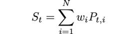
is stationary.
Given the vector w (“w_vec”) and the processes P_i, encoded as a matrix (“p_mat”) with one process in each column getting S is very simple:
Dickey-Fuller statistic, direct estimation
The first thing we will address is optimizing the function call speed. Usually, to calculate the Dickey-Fuller test, we would do OLS regression. That is expensive. Instead, we use a direct estimation for the test statistic:
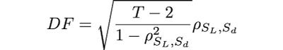
where ρ_SL,Sd is the correlation (Pearson) for the lagged S series (S_L) and the differenced S series (S_d). Notice that the sample size of both S_L and S_d is T.
If you want more details about the above result, check my previous story with the mathematical proof.
Using the Dickey-Fuller statistic in this form is faster since calculating the correlation coefficient is computationally more efficient than OLS matrix inversions and multiplications. Furthermore, it has another advantage; the dependence of the statistic on the vector w is clear. Since the correlation is:

and the covariance and the variances of S_L and S_d can be written as quadratic forms using covariance matrices and the w vector, i.e.

and

where V_L is the covariance matrix of the lagged P_i time series, V_d is the covariance matrix of the differenced P_i time series, V_L,d and V_d,L are cross-covariance matrices for the lagged and differenced time series, they are defined as:

with the property that:

the T superscript denotes matrix transpose.
Coding the talk, we initialize the “_SInit” object with the essential variables we will need through the calculations:
Then another object, “_PCovMatrices” with the covariance matrices we will need:
and lastly, the standard deviations object for the lagged and differenced S series:
With the initial objects coded we can now state our objective function, the Dickey-Fuller statistic direct estimation:
The gradient
The gradient of DF (Dickey-Fuller) with respect to w is:
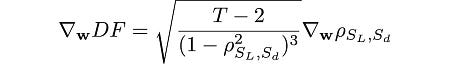
and the gradient of the correlation is:

Using the gradient of the quadratic form, the gradients of the standard deviations and the covariance are:
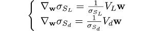
and

Hence,

Coding the gradient:
The Hessian matrix
To get the Hessian matrix, we will use tensor calculus because we will need to deal with the derivative of a matrix with respect to a vector and funky math of the sort, so tensor calculus is best suited.
We will use Einstein’s summation convention of repeated indices; sum signs would complicate everything further because we have many indices. Furthermore, we will use the following simplification:

In the covariance matrices, we will use the subscript field for indices:

Indices will be written in greek letters to differentiate them from other subscripts and superscripts.
The Hessian is:

where

is the gradient of the correlation, in vector calculus notation

assuming the gradient is a column vector.
We need to calculate the Hessian for ρ. To wit, let's define two matrices that we will use:
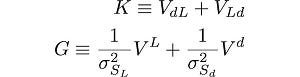
and a 4-tensor:

Then the gradient of ρ (already in vector calculus notation in the previous section) in tensor calculus notation is:

is difficult not to love the elegance of tensor calculus.
Finally, the Hessian for ρ is:
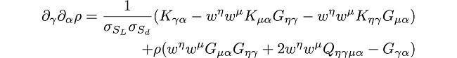
Although it looks like the equation of a collapsing black hole in general relativity (just kidding), coding this in Python is very simple, thanks to NumPy’s “einsum”:
Minimization
The minimization code block is very straightforward once we have the objective function, the gradient, and the Hessian. Essentially we wrap SciPy’s minimize function with the arguments of our cointegration problem:
- “p_mat” is the P_i processes matrix.
- “w_vec_init” is an initial guess for w_vec. Don’t worry if you don’t supply one; a random guess will be generated.
- “method” can only take two values, either “trust-krylov” or “trust-exact”.
Note: This is not a global optimizer, so giving an initial w vector is essential for convergence. In some problems, the randomly picked vector is enough for convergence. However, it would be best to generate a better initial guess for your particular situation.
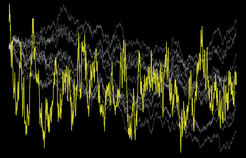
We will generate discretely sampled correlated Brownian motions (unit root processes) and use this matrix as “p_mat” to test the algorithm. If you don’t know about Brownian motions or how to generate them, don’t worry; check out my previous story on the subject. We will use the code from that story to generate the “p_mat”, so save the code from the Brownian motion story as “brownian_motion.py” and put it in the same directory where you run the following code.
Minimize and plot:
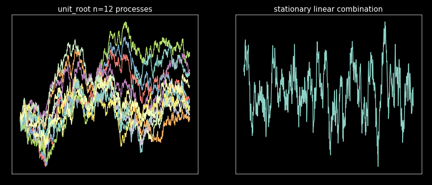
Everything worked as intended.
Code Summary
For completeness, here is all the code developed in the story. The code you need to get the cointegrating vector by minimizing the Dickey-Fuller test statistic:
Final words
The optimization algorithm developed worked as intended. The speed is not as good as eigendecomposition algorithms but comparable. And it is very robust and reliable.
However, the only downside is the choice of an initial guess for the cointegrating vector. I’ve seen that the method is very forgiving for a poor choice of the initial guess; most of the time, the random initial guess works great. Nevertheless, making a good choice can increase the speed and reliability of the solution. Remember, this is a local optimizer, not a global optimizer.
Finally, with the gradient and the hessian, it is simple to extend this code into a constrained optimization, which is more suitable for real-world problems. Constraints can be easily added to this method. The eigendecomposition methods would have to be rewritten to accommodate constraints.
References
[1] M. L. de Prado, D. Leinweber, Advances in cointegration and subset correlation hedging methods (2012), Journal of Investment Strategies, Vol. 1, №2, pp. 67–115
I hope this story was useful for you. Follow me on Medium and subscribe if you’d like more stories like this.
Get an email whenever Diego Barba publishes.
If I missed anything, please let me know. For any doubts, criticisms, etc., leave a comment.
Dickey-Fuller Optimization: Tackle Time Series Cointegration Head-on was originally published in Towards Data Science on Medium, where people are continuing the conversation by highlighting and responding to this story.
from Towards Data Science - Medium https://ift.tt/eMNiDar
via RiYo Analytics


No comments