https://ift.tt/AonxJZ1 A Quick-Start Guide to A/B Testing A step-by-step approach to finding valuable insights Photo by Braden Collum o...
A Quick-Start Guide to A/B Testing
A step-by-step approach to finding valuable insights

Introduction
So you’ve been tasked to set up a marketing A/B test and don’t have a lot of time to figure things out. Here is a quick start guide on how to do it when the main metric to improve is a proportion: click-through rate, conversion rate, open rate, reply rate…
1. Define your null hypothesis and choose your significance level
The first step in the process is to define what hypothesis you want to test. More often than not, you are hoping that a change in a landing page, a banner ad or an email copy (the B version, or treatment) performs better than the current version (the A version, or control group). So the rule is: you define your null hypothesis as what you hope to be false. For instance, you want to test a new colour for a submit button and hope that this button will generate more form submissions than the old one. Your null hypothesis (H0) is that the new button will perform worse or the same as the existing one and the alternative hypothesis (H1) is that the new button will perform better (so: generate a higher click-through rate).
We are testing for the difference between two proportions pA and pB so:
H0: pB ≤ pA or, equivalently, pB-pA≤0 ; this is our null hypothesis, what we hope to show is false: the proportion of events — clicks, conversions, replies — in the B version (pB) is lower or the same as the proportion of events in the original A version (pA)
H1: pB > pA or pB-pA>0 ; our alternative hypothesis, the new version B shows a higher proportion of events than A.
Finally, you have to choose a significance level, usually called alpha, which represents the probability of making a Type I error (adopting the new version when it is in fact performing worse). Commonly-used levels are 5% or 1%, which roughly means that if you run 100 tests a year you should expect on average that for 5 (or 1, depending on your alpha value) of them you would make the wrong decision and implement a change that is not actually improving things.
2. Randomise your users
This is a crucial step and it is very important your tech teams understand the requirement as it happens too often that, to simplify the process, users are not randomly shown version A or B. For instance, a 4-weeks test could be split into 2 weeks with the current version and the following 2 weeks with the new version, or morning vs. afternoon, or one browser vs another one. This is NOT good practice and will most probably introduce biases in your data and as a result, it is likely your conclusions won’t apply to your whole audience. It is also important to be aware of the unit of observation: are we basing it on devices, cookies, IPs or logged-in users?
3. How Many Users? With great Power Comes Great Sample Size
You should ensure that your test design has enough power (a commonly used value is 80%) but what is the Power of a statistical test and how can we choose an adequate sample size that gives us enough power? If you don’t have time to read about the theory, skip to the end of this section for a quick rule of thumb and an online calculator (and even a mobile app!)

To understand power, we need to understand what Type I and Type II errors are. A Type I error is when we reject the null hypothesis when it is in fact, true. For example, imagine our new banner version (B) performs worse than our original design (A) but due to randomness, the data shows that B performs significantly better and so we reject our null hypothesis erroneously. By definition, this is meant to happen 5% of the time on average if you use a significance (alpha level) of 5%.
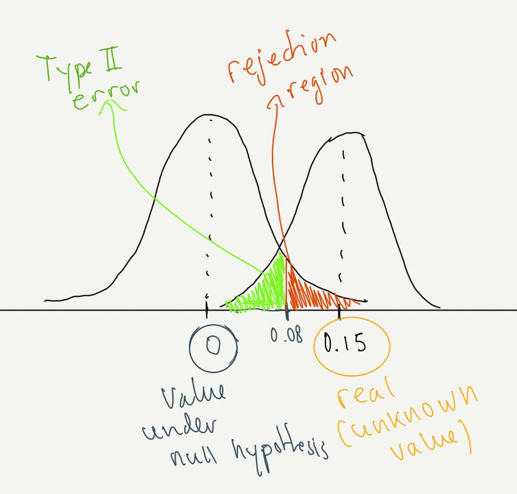
A Type II error is not rejecting the null hypothesis when we actually should. In our example, imagine version B performs better than version A but our test doesn’t offer enough power to reject the null hypothesis and so we keep version A and lose an opportunity to improve performance. As we can see in the (very rough) image below, under a null hypothesis of pB-pA=0, we would reject that null hypothesis if the observed value is greater than 0.08 (the region in red). If the real (and unknown) difference were actually 0.15, we would fail to reject any value falling in the green region and so we wouldn’t be able to determine that version B is superior to version A. This is the probability of making a Type II error and the power of our test is one minus that probability.
Let’s look at the following hypothetical results, we created a simulation in Python to illustrate the point with a binomial data generating process with probability .005 for group A and .0075 for group B:
from scipy.stats import norm
import numpy as np
# Let's define our sample size
n=500
p_a = .005  # real underlying probability of each trial for version A
p_b = .0075 # same for B
# We generate the random binomial samples (number of clicks for 500 ad impressions in each group)
s_a = np.random.binomial(n, p_a, 1)
s_b = np.random.binomial(n, p_b, 1)
# calculate pooled p
p=(sum(s_b)+sum(s_a))/(2*n)
print(p)
# calculate standard error
se=np.sqrt(p*(1-p)*(2/n))
print(se)
# calculate test statistic
z=(s_b/n-s_a/n)/se
print(z)
# get the p-value
print(1-norm.cdf(z))
With a sample size of 500 we obtained the following results (feel free to run your own tests), p_A=0.004, p_B=0.01 with a p-value of 0.32. We cannot reject the null hypothesis, even though we know we should, as the samples were generated with known underlying probabilities (and pB was higher than pA). This is clearly a Type II error.
How can we reduce that risk? It’s fairly simple, we need to increase our sample size. Using the same code, but changing the sample size to 100,000 we get: p_A=0.0048, pB=0.0074 and a p-value well below 0.001. But we used the same underlying process, we only changed the sample size!
The formula to calculate a big enough sample relies on the concept of effect size, or: what is the minimum difference you want to be able to detect (and that makes business sense)? It could be, for instance, a difference of at least 0.05 percentage point, bringing an existing conversion rate of 0.1% up to 0.15%. Of course, the required effect size would vary depending on the business sector and the applications, but it needs to be somewhat justifiable to the management teams.
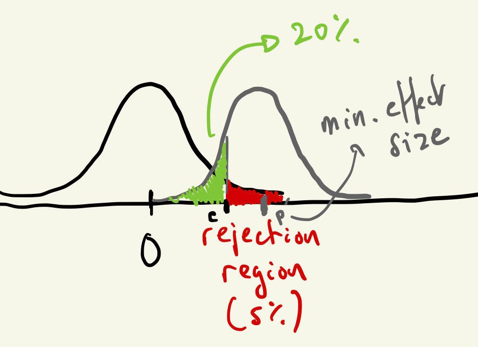
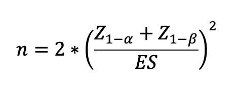
The formula to calculate the sample size uses the significance level (alpha), the power level (1-beta) and the effect size (ES), you can find a very good explanation on how the formula is derived here (https://online.stat.psu.edu/stat415/lesson/25/25.3), we are essentially looking for a value c that is both a cut-off value for a rejection region and for our probability of getting a false negative (see figure below)
So, the formula is as follows:
With ES as:
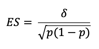
Delta being the minimum difference you want to be able to detect and p the overall average proportion across the two samples (A and B).
It should be easier with an example: you are running a banner (A) campaign with a CTR of 0.5% and you want to test a new banner (B). You are only interested in a minimum 50% increase in CTR, so a new improved CTR of 0.5%*1.5=0.75%, an absolute difference of 0.25 percentage points. What is the minimum number of impressions you need to run in each version to be at least 80% confident to detect a difference at the 5% significance level?
a) The significance level is 5% so our Z(1-alpha) value is 1.645
b) The required Power is 80% so our Z(1-beta) is 0.842
c) Our overall (average) proportion p is (0.005+0.0075)/2=0.00625
d) And our effect size ES is (0.0075–0.005)/sqrt(0.00625*0.99375) =0.03172
So our n = 2*[(1.645+0.842)/0.03172]² = 12,296 impressions on each banner
If we run our Python code 12,296 times we see that with that sample size, we get p-values>0.05 on average 20% of the time!
Finally, a useful rule of thumb to calculate n for a power of 80% and a significance level of 5%:

You can also use this online sample size calculator:
Or download the A/B Buddy app on Android or iOS.
4. What test to use for the difference between proportions?

When the test is over, the first step is to compare the results, which version, A or B, performed better? But also, are the differences between the two versions significant or due to chance? In comes statistical testing, there are several ways to test if the observed differences are statistically significant, some posts on TDS suggest Fisher’s exact test or a Chi-square test but we are going to use a Z-test. The main idea behind the Z-test that if we take many samples from a binomial distribution, the proportion of successes would be normally distributed (ideally we also want to make sure that n*p>5). So we need to answer the question: what is the probability of getting the existing results if the null hypothesis were true? We simply need to calculate a test statistic which we know follows a standard normal distribution and find the probability of observing a value as least as extreme if version B were indeed worse or the same as version A.
Here is a simple step by step procedure with an example. Say you run a test between two different advertising banners and after running the test for a few days you get the following results:
Version A: 12,000 impressions and 18 clicks, which is a CTR of 0.15% (18 / 12,000 = 0.0015)
Version B: 11,800 impressions and 23 clicks, or a CTR of 0.195%
Step 1: calculate the pooled proportion, p

In our example we have nA=12,000, pA=0.0015, nB=11,800 and pB=0.00195 which gives us:
p= (18 + 23)/(12,000+11,800) = 0.00172, or 0.172%
Step 2: calculate the standard error of p, SE
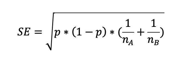
Which gives: sqrt[0.00172 * 0.998 * (1/12,000+1/11,800)] = 0.00054 or 0.054%
Step 3: calculate the test statistic, Z

So Z = (0.00195–0.0015)/0.00054 = 0.833
Step 4: find the probability of getting that particular value.
Use Python, R or Excel to get your p-value.
Python
from scipy.stats import norm
p_value = 1-norm.cdf(zvalue)
Excel
1-NORM.S.DIST(zvalue,TRUE)
R
p_value <- 1 - pnorm(zvalue,mean=0,sd=1)
We get a p-value of 0.202 so we cannot reject the null hypothesis and as a result cannot establish that version B is performing better than version A.
Also good to know
A/A testing
What is A/A testing and why should you care? A/A testing is basically running the same version of a website, banner ad or email copy twice within a test design to assess the randomisation process and the tools you are using. The users in each group see the same thing but you want to compare the results and see if the difference in performance can be attributed to chance. If the differences are statistically significant it could reflect issues with your test design or processes that you’ll have to investigate. It is also worth noting that on average you should expect to see false positives in roughly 5% of the cases if your significance level (alpha) is 5%.
Sequential testing
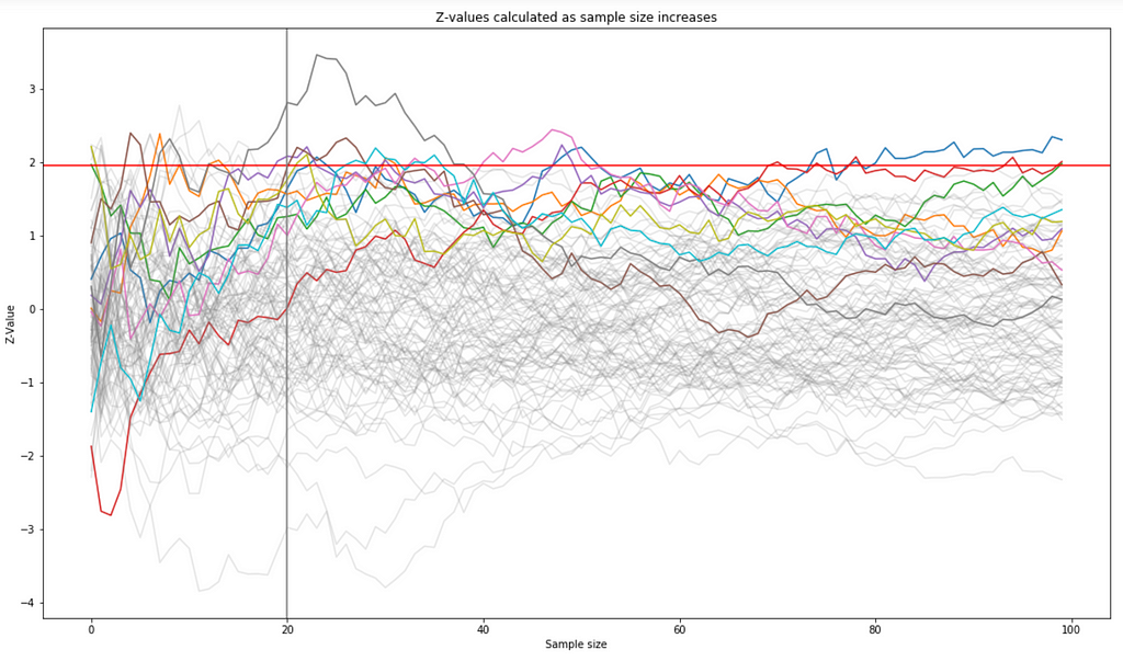
Can you stop before the end of a planned test if the results seem to indicate a clear improvement or a when the new version being tested is clearly underperforming? The issue with “peeking” is that it tends to generate more false positives, as can be seen in the simulation below. We generate 100 random samples with the values of the null hypothesis. With a significance level of 0.05, we can see that 3 samples out of 100 would lead us to reject the null hypothesis, which is not far of the expected value of 5 samples. But if we start peeking and calculating z-values after the sample reaches a size of 20, we would have rejected all the coloured lines in the graph below (10 out of 100).
Abraham Wald—famous for his survivorship bias observation on warplanes — and his colleagues at the Statistical Research Group, designed a methodology to speed up the testing process, the Sequential Probability Ratio Test. It requires an understanding of the concept of likelihood ratio and you can find an excellent explanation of the method here:
Experiments, Peeking, and Optimal Stopping
Bayesian approach
So far we have covered the “traditional” frequentist approach but the Bayesian framework is also very popular in the context of A/B testing. It presents some advantages:
a. It is easier to communicate results to stakeholders in the business with the Bayesian framework, as unlike the frequentist method, we can can talk in terms like “the probability that B is better than A”.
b. Bayesian A/B tests tend to be faster and give more flexibility when deciding when to stop the experiment
c. One of the issue with the frequentist approach is that we reject a version based on the p-value but without directly taking into account the magnitude of the effect. Bayesians use of a “loss function” that treat small errors as less serious than big ones and help decide on a loss threshold and a risk-level they are comfortable with. This matches the decision-making process in other business areas.
At a very high level, the process involves choosing a prior distribution for the rate we are experimenting on (most likely a Beta distribution). The prior allows the inclusion of “expert opinion” or past data into the model. We then run the test (effectively on a binomial variable in our case) and combine the results with the prior to obtain a posterior distribution for pA and pB. Monte-Carlo simulations can then be run to obtain probabilities that pB>pA and also build the aforementioned loss function.
You can read more about Bayesian A/B testing in this excellent white paper by Chris Stucchio.
Multi-armed bandit algorithms (MAB)
Named after a classical mathematical optimisation problem where a gambler needs to maximise his winnings on a set of slot machines with different (unknown) payouts. The MAB algorithm is an optimisation process that changes the allocation of impressions to the best-performing version and so maximises the number of conversions at the expense of statistical validity, as results can become difficult to analyse due to that optimisation process. It answers the explore vs exploit dilemma. More about MAB here:
A/B testing — Is there a better way? An exploration of multi-armed bandits
Segmented A/B tests
Instead of working with averages and show every audience an overall optimal design, you can test for specific segments and personalise the optimisation process to subgroups (based on demographics, location, etc). Here is good blog post by Yaniv Navot.
ROI considerations
Obviously, before running an experiment it is important to factor in the cost of running the experiment, implementing a new version vs the business impact. The ROI is calculated as follows:

To take an example, if a new version of website increases our $1 million yearly sales by 1% but the cost of testing and implementing the new version is $12,000, is it really worth the effort? You can check Georgi Georgiev’s ROI calculator, part of his A/B planning and analysis tool:
https://www.analytics-toolkit.com/ab-test-roi-calculator/
External validity
External validity refers to how generalisable our results are. There are many factors we cannot easily control for, such as changes in our audience, actions from our competitors, changes in the economy, etc. and they might all affect results after the experiment. Two concepts you need to be aware of are the novelty and learning factors. Those two effects refer to the fact that loyal users of an e-commerce site for example might feel a bit disoriented when seeing a different version of the website and as a result affect the KPI we are tracking (negatively). The key here is we are expecting those users to adapt over time and so what we are observing during a short test wouldn’t apply for a larger timeframe. Three Google employees (Hohnhold, O’Brien and Tang) put together a “model that uses metrics measurable in the short-term to predict the long-term”, see paper here or a video presentation here.
Testing more than two versions: A/B/n testing
Finally, if you want to test more than 2 versions of your website, banner or email copy, you need to take into account issues around Family-wise error rate (FWER) and adjust the p-values accordingly. There are several options such as the Bonferroni correction, the Dunnet’s correction or the Sidak’s correction.
It is another vast subject and you can find more information here.
Good luck!

Recommended links and books
Kohavi, R., Tang, D., & Xu, Y. (2020). Trustworthy Online Controlled Experiments: A Practical Guide to A/B Testing. Cambridge: Cambridge University Press.
Georgi Zdravkov Georgiev (2019), Statistical Methods in Online A/B Testing: Statistics for Data-driven Business Decisions and Risk Management in E-commerce. Independently published.
- Sample Size Calculator
- Exploring Bayesian A/B testing with simulations
- A/B testing — Is there a better way? An exploration of multi-armed bandits
A Quick Start Guide to A/B Testing was originally published in Towards Data Science on Medium, where people are continuing the conversation by highlighting and responding to this story.
from Towards Data Science - Medium https://ift.tt/aTVQyAz
via RiYo Analytics

ليست هناك تعليقات