https://ift.tt/yFHaCbB psmpy: Propensity Score Matching in Python — and why it’s needed image by author When we try and answer quesions...
psmpy: Propensity Score Matching in Python — and why it’s needed
When we try and answer quesions like:
‘Does taking beta blockers reduce risk of heart attacks?’
‘Does smoking cause cancer?’
‘Do STEM programs in elementrary schools encourage more students to go into the sciences?’
We often attempt to answer that question using randomized control trials (RCTs) which we use to perform A|B testing. We try and control the kind and number of variables that might affect this outcome to ascertain if some intervention (or lack thereof) has a potential causal link to the outcome! In the 3rd question posed above you might want to control for socioeconomic status (SES), neighborhood or parental education. In the case of a medications, we may want to consider: age, sex, race, underlying/pre-exiting health conditions etc. Enter RCTs…
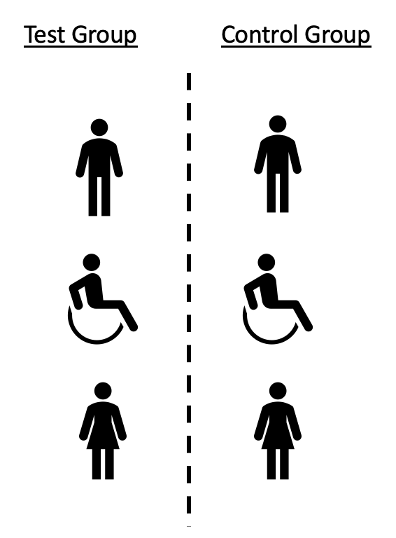
RCTs are prospective (planned and outcomes occur in the future) and patients are usually matched (sharing similar features — SES, age, etc.) 1:1 for all the variables we want to control for, where 1 receives the intervention and 1 does not.
Issues with RCTs:
- Expensive $$$
- Don’t scale (as we increase number of variables we want to control for)
- Patient/participant drop out
- May ultimately not yield meaningful results
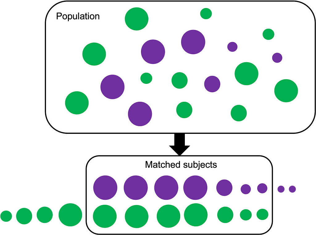
Propensity score matching (PSM) is a statistical technique used with retrospective data that attempts to perform the task that would normally occur in a RCT. So it works as follows:
- A large group of patient/participant data that have already been collected (historical data remember?) — age, sex, SES, weight. These are covariates. Often our covariates are potential confounders that could bias our results. The intervention = taking the drug (yes/no) and follow up on our outcome = heart attack (yes/no). Imagine electronic health record data!
- Try to find someone who is a ‘match’ for Mrs. X who has taken the medication who has many of the same covariates as she does but didn’t take the medication [2]. And we need to do this for as many people as possible to create a cohort of treated/not treated.
- We fit a series of logistic regressions to our population where all our ‘predictor’ variables are our covariates (age, sex, weight), and we are trying to predict our intervention. Unlike most machine learning tasks we don’t calculate the accuracy here. It is the predicted proability we are interested in. Using indexes (participtant IDs) we know who came from which intervention group, treatment or control.
- Using that probability calculated we find a closest match from the opposing group. E.g. Mrs. X had a probability (propensity) score of 0.4 and received the medication and Mr. Y did not received the medication and had a proabability score or 0.42. K-nearest neighbors is often used to find these matches and we can do 1:1 matching or 1:many matching (duplicates allowed). Matches may be excluded if the difference in the proababilities is deemed to be too large.
- Effect sizes are a measure of how well we’ve been able to control for all these covariates [4]. We want them as small as possible, so any changes in the outcome can be attributable to the the intervention performed, giving us a potential causal link. So we want to calculate these before and after matching to understand our data!
- After matching we have identified a subgroup out of our population to study, we can investigate how our intervention affected our outcome. While the intervention is a binary one the outcome can be continuous or binary, we just need the correct statistical test.
Benefits of PSM:
- Fast
- Cheap — it’s a mathematical match
- No issues w/ patient drop out (since historical data)
- Scales — can have as many covariates as we like!
- Repeat the process easily and change variables at a whim (assuming we have the data to support the endeavor)
Downsides to PSM:
- a mathematical match may not be an epidemiological match
A mathematical match means Mrs. X who is a 68 y.o. female who received the medication, may not necessarily be matched to a female 68 y.o. who did not receive the medication. Using PSM, she may have matched to a 55 y.o. male if other covariates in the model with larger weight are similar.
Although not as accurate as RCTs, as more data are moved into the digital realm, PSM can offer insights into real world settings. It can automate and detect meaningful results without the hassle or cost of an RCT.
As there currently does not exist a widely applicable and well performing PSM library in python, enter — PsmPy! https://pypi.org/project/psmpy/
Features of this library include:
- Additional plotting functionality to assess balance before and after
- A more modular, user-specified matching process
- Ability to define 1:1 or 1:many matching
Installation
PsmPy is available on pypi.org and can be installed through pip in terminal:
$ pip install psmpy
Data Prep
Read in your data.
# import other relevant libraries (that you want)
# set the figure shape and size of outputs (optional)
sns.set(rc={'figure.figsize':(10,8)}, font_scale = 1.3)
# read in your data
data = pd.read_csv(path)
Import psmpy class and functions
Import the PsmPy library into python and the 2 other supporting functions:
CohenD calculates the effect size and is available to calculate the effect size exerted by variables before and after matching. The closer this number is to 0 the more we have been able to effectively control the covaiates
from psmpy import PsmPy
from psmpy.functions import cohenD
from psmpy.plotting import *
Instantiate PsmPy Class
psm = PsmPy(df, treatment='treatment', indx='pat_id', exclude = [])
Note:
- PsmPy - The class. It will use all covariates in the dataset unless formally excluded in the exclude argument.
- df - the dataframe being passed to the class
- exclude - (optional) parameter and will ignore any covariates (columns) passed to the it during the model fitting process. This will be a list of strings. It is not necessary to pass the unique index column here.
- indx - required parameter that references a unique ID number for each case in the dataset.
- outcome - required parameter that represents a binary outcome of interest (0 or 1) and differentiates the treatment from control or success/fail of each group.
Predict Scores
Calculate logistic propensity scores/logits:
psm.logistic_ps(balance = True)
Note:
- balance - Whether the logistic regression will run in a balanced fashion, default = True.
There often exists a significant class imbalance in the data. This will be detected automatically. We account for this by setting balance=True when calling psm.logistic_ps(). This tells PsmPy to create balanced samples when fitting the logistic regression model. This calculates both the logistic propensity scores and logits for each entry.
Review probabilities/logits in dataframe:
psm.predicted_data
Matching algorithm
Perform KNN matching
psm.knn_matched(matcher='propensity_logit', replacement=False, caliper=None)
Note:
- matcher - propensity_logit (default) and generated in previous step alternative option is propensity_score, specifies the argument on which matching will proceed
- replacement - False (default), determines whether macthing will happen with or without replacement, when replacement is false matching happens 1:1
- caliper - None (default), user can specify caliper size relative to std. dev of the control sample, restricting neighbors eligible to match
Graphical Outputs
Plot the propensity score or propensity logits
Plot the distribution of the propensity scores (or logits) for the two groups side by side.
psm.plot_match(Title='Side by side matched controls', Ylabel='Number of patients', Xlabel= 'Propensity logit', names = ['treatment', 'control'], save=True)
Note:
- title - 'Side by side matched controls' (default),creates plot title
- Ylabel - 'Number of patients' (default), string, label for y-axis
- Xlabel - 'Propensity logit' (default), string, label for x-axis
- names - ['treatment', 'control'] (default), list of strings for legend
- save - False (default), saves the figure generated to current working directory if True
This is demonstrated using the Heart Disease Health Indicators Dataset [3].
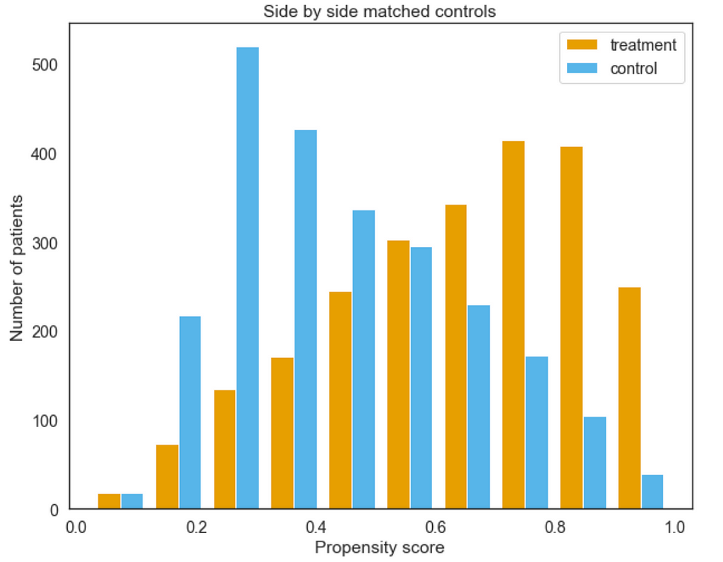
Here we can see the treatment and control groups plotted against one another (after matching). The nearer the two distributions mimic one another the better our matching is.
Plot the effect sizes
psm.effect_size_plot(save=False)
Note:
- save - False (default), saves the figure generated tocurrent working directory if True
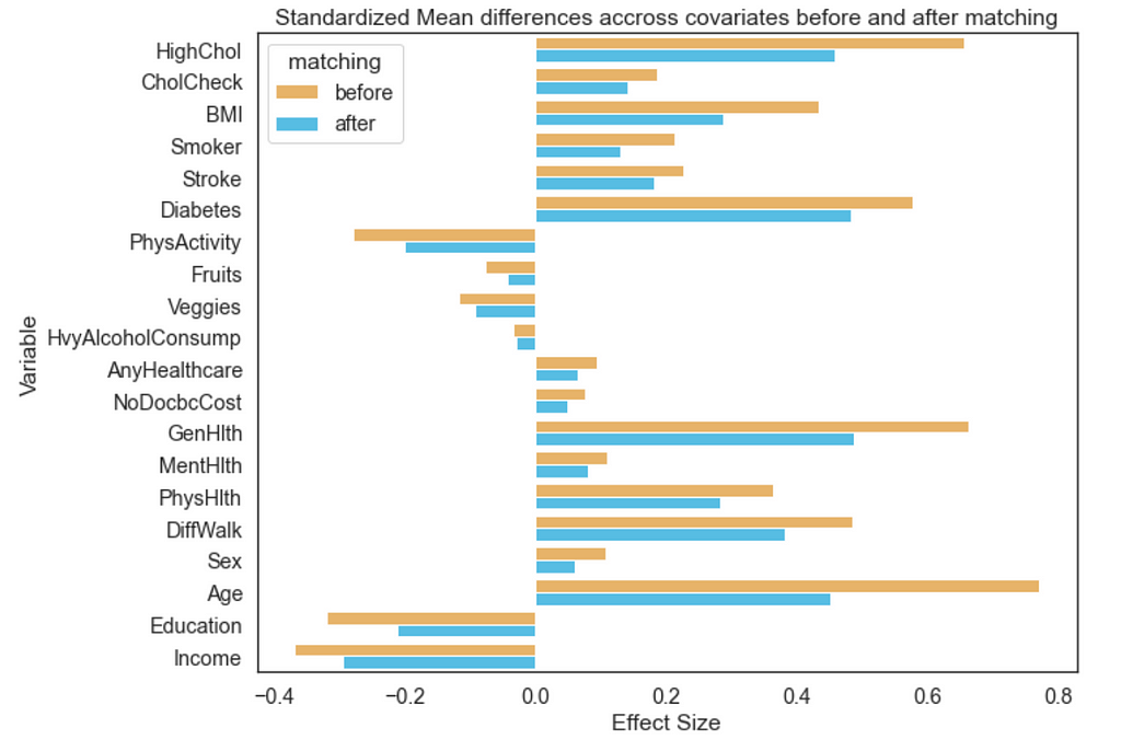
We can plot effect sizes using the code above. Here we can see the effect size (calculated using Cohen’s D) which is a modified Chi square test. This is performed on each variable before and after matching for the cohorts.
Extra Attributes
Other attributes available to user:
Matched IDs
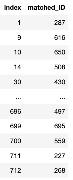
psm.matched_ids
- matched_ids - returns a dataframe of indicies from the minor class and their associated matched index from the major class psm.
Note: That not all matches will be unique if replacement=False
Effect sizes per variable
psm.effect_size
- effect_size - returns dataframe with columns 'variable', 'matching' (before or after), and 'effect_size'
Note: The thresholds for a small, medium and large effect size were characterized by Cohen [4]. Where relative size effect are classified as: small≤ 0.2, medium≤ 0.5, large≤0.8.
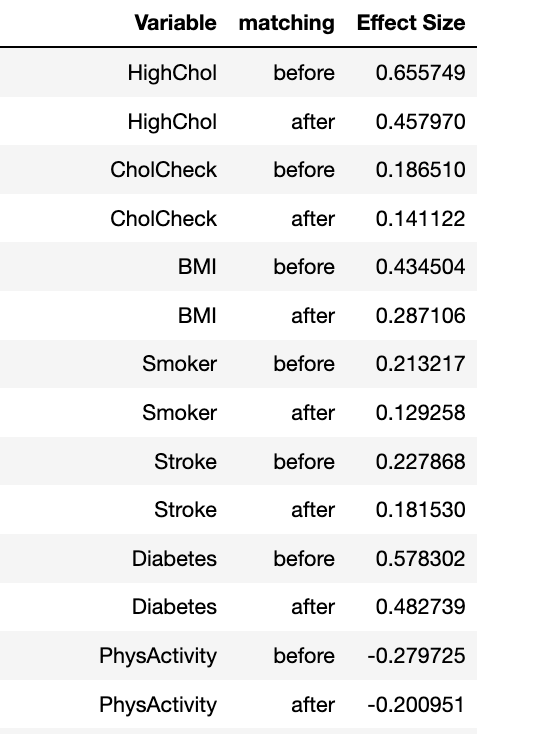
Ideally, ‘after’ matching the effect size exerted by the variable should be smaller than the before. The closer these effect sizes are to 0 the less our outcomes of interest will depend on that covariate.
Currently there does not exist an easy to use PSM technique in a Python environment. There exists the package MatchIt in R environment [5] and another alternative in SPSS. The MatchIt package offers a few rudimentary plotting features, however, psmpy is open source (unlike SPSS) and offers easy to use/customize visually pleasing figures to determine how ‘good’ a match was, and several class attributes to enable end users to get at the raw data that is calculated from the algorithm.
Citing this work! : )
A. Kline, Y. Luo, PsmPy: A Package for Retrospective Cohort Matching in Python, (accepted at EMBC 2022) [1]
Contact for preprint!
References
[1] A. Kline, Y. Luo, PsmPy: A Package for Retrospective Cohort Matching in Python, (accepted at EMBC 2022), doi to follow when available
[2] Paul R. Rosenbaum & Donald B. Rubin, “The central role of the propensity score in observational studies for causal effects”, 1983
[3] Heart Disease Health Indicators Dataset, https://www.kaggle.com/datasets/alexteboul/heart-disease-health-indicators-dataset
[4] J. Cohen, “A Power Primer”, Quantitative Methods in Psychology, vol.111, no. 1, pp. 155–159, 1992
[5] Ho, D. E. et. al, “MatchIt: Nonparametric Preprocessing for Parametric
Causal Inference”, Journal of Statistical Software, vol.42, no. 8, 2011
doi:10.18637/jss.v042.i08
psmpy: Propensity Score Matching in Python! was originally published in Towards Data Science on Medium, where people are continuing the conversation by highlighting and responding to this story.
from Towards Data Science - Medium https://ift.tt/CHd7Sca
via RiYo Analytics


No comments