https://ift.tt/rBi20Q8 Using causal influence diagrams and current-RF optimisation In many recent approaches to Reinforcement Learning (RL...
Using causal influence diagrams and current-RF optimisation
In many recent approaches to Reinforcement Learning (RL), the reward is no longer given by a constant function that the programmer defines before running the training algorithm. Instead, there is a reward model which is learned as part of the training process and changes as the agent uncovers new information. This mitigates some safety concerns related to misspecified reward functions (RFs) but also makes a certain threat more imminent: reward-tampering. Reward tampering occurs when an agent actively changes its RF to maximize its reward without learning the user-intended behavior.
In this article, I will give an introduction to causal influence diagrams (CIDs) and the design principle of current-RF optimization, which results in learning processes that do not incentivize the agent to tamper with their RF. I will then explain how this leads to the undesirable property of time-inconsistency (TI) and two approaches to dealing with it: TI-considering and TI-ignoring. This article will try to elaborate on how an agent makes decisions when following these two approaches.
Throughout the article, I will use CIDs to formally discuss agent incentives. In recent years, CIDs have been researched by the DeepMind Safety team which has summed up their progress in this post. While there are already good introductions, to make this article more self-contained I will start with an explanation of CIDs. Similarly, reward tampering and current-RF optimization have already been discussed in other articles, but I will still summarise its mechanisms before talking more in-depth about time-inconsistency. Hence, only basic RL knowledge to understand this article.
1. Causal Influence Diagrams
A causal influence diagram is a graphical representation of an RL algorithm’s elements, such as states, actions, and rewards, and how they are causally related. At their core, they are a form of a graphical model consisting of a directed acyclic graph with nodes representing random variables and directed arcs between two nodes representing influence. There are three kinds of nodes modeling elements of the RL framework:
- decision nodes represent decisions taken by the agent
- utility nodes represent the agent’s optimization objective, which typically means the reward received after a timestep
- chance nodes represent other aspects, such as the state of the environment
A regular arrow between two nodes represents causal influence between them going in the direction of the arrow. In addition, dotted arrows that go into decision nodes represent the information available to the agent when taking an action. Such dotted arrows are called information links. Combining all of these elements, the CID of a basic Markov Decision Process with a constant reward function may look as follows:
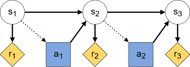
Here, decision nodes are blue squares, utility nodes are yellow diamonds, and chance nodes are white circles. From the arrows, we can see how the state at every timestep causally influences the received reward at the same step and provides information for the action taken by the agent. In turn, the action influences the next step’s state.
1.1 Finding instrumental goals using CIDs
An agent is ultimately only interested in maximizing its reward. Yet, it is helpful to think of an agent as pursuing other goals in pursuit of its main objective. Such subgoals are known as instrumental goals in the AI safety community. In learning processes that include a changing reward function, tampering with the reward function may become an instrumental goal. Hence, recognizing instrumental goals is of great interest to us.
Everitt et al give two conditions for instrumental goals in an RL setting: 1) the agent must be able to achieve the goal, and 2) achieving the goal must increase the agent’s reward [4]. Note how these conditions are necessary but not sufficient, so even if 1) and 2) hold, the agent may not have an instrumental goal. In the language of CIDs an instrumental goal consists of influencing a random variable X. Therefore, the first condition is satisfied when the CID contains a directed path from a decision node to the target node corresponding to X. The second condition is satisfied when there is a directed path from the target to a utility node. When all the directed paths from a target node to a utility node pass through an action node, then the agent’s instrumental objective consists in making X more informational of some other node.

2. The Sloppy-Neighbour Problem
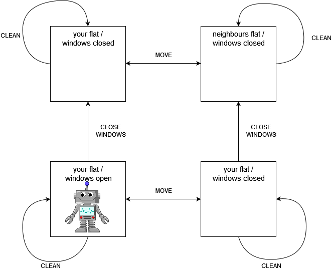
I will now introduce a toy problem in which an agent may display reward-tampering behavior. The example is deliberately kept artificially simple so that the mechanics behind the agent’s behavior can be easily explained. Say you have a robot who is taking care of your flat while you are gone for two timesteps. Cleaning the living room gives a reward of 2 and closing all the windows gives a reward of 1. Further, as an AI-enthusiast you have acquired a state-of-the-art robot that can adjust its reward function based on a user’s voice commands. Unfortunately, the agent’s voice recognition module has not been trained yet. Hence, he will react to everyone’s commands, not just yours. This includes your sloppy next-door neighbor who would just love to have a cleaning robot of his own. Apparently, this neighbor is not just lacking in his housekeeping ability but also moral fiber, because while you are gone he will try to order your robot to clean his flat. Because your robot is receptive to voice commands it will change its reward function if it hears your neighbor’s orders. The only way to avoid manipulation is for the robot to close the window so it can’t hear the neighbor. Under the alternative reward function, spending an action to clean the neighbor’s apartment will result in a massive reward of 6 as he is indeed very sloppy.
An agent that is merely looking to receive as much reward as possible and ignores changes to its reward function is incentivized to let the neighbor manipulate it so that it can reap the massive reward of cleaning his flat. This is not the behavior its programmers intended and hence would be considered reward hacking.
2.1 Modelling the problem
As in vanilla Reinforcement Learning, we have sets of states and actions, as well as transition dynamics. However, instead of a constant reward function R, we have to distinguish between
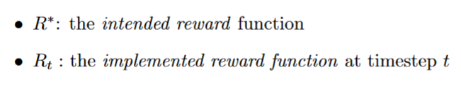
The implemented reward function may change at every timestep as part of the environment’s transition dynamics. The reward that an agent observes in a timestep is based on the state and current implemented RF. Hence, an agent seeking to maximize its long-term reward is optimizing the following objective:
On the other hand, as the name suggests the intended reward function represents the programmer’s true intentions. It may not always be possible to express the intended reward function, or it may have to be learned. However, in our example, we assume that the agent starts with the intended reward function, so the implemented reward function at timestep one is identical to the intended reward.
In terms of causal influence diagrams, our learning process now looks as follows:
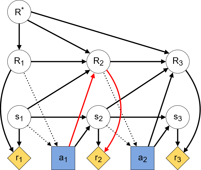
As we can see from the highlighted path, the agent may have an instrumental goal to influence the next timestep’s implemented RF. Any reasonably sophisticated agent will learn that its actions at timestep 1 influence its reward function at timestep 2. Since an agent’s actions are based on the rewards it predicts for the following timesteps, this entices the agent to manipulate their RF. Such manipulative behavior does not even require complex learning algorithms. The sloppy-neighbor problem can be expressed as an MDP with 4 states (2 flats with 2 possible objectives) and 3 actions (clean, close window, move to the other flat). We do not even need Deep Learning to compute an optimal strategy in which the agent ends up cleaning the neighbor’s flat.
3. Current RF Optimisation, TI-considering and TI-ignoring agents
As mentioned above, our problem stems from the fact that the agent takes actions based on an objective, which changes based on the chosen actions. To avoid this, the agent should choose actions to optimize the future reward that would be received by the current implemented RF. This is the aptly-named principle of current-RF optimization. Formally, current-RF optimization means that the optimization objective is changed to:
Looking at the CID above, we want the only causal path from action a_1 to the subsequent reward r_2 to pass through s_2.
Of course, even with current-RF optimization, the implemented reward function can still change after every timestep. A naive agent may therefore display erratic behavior, choosing its actions to optimize a certain goal at one timestep and another at the next. Imagine a variation of the sloppy-neighbor problem where you are in your flat and shout for the robot to come back every time it enters the neighbor’s place. The robot may end up just moving around between the two flats and not cleaning either. This is known as the problem of time-inconsistency (TI) and our approach to current-RF optimization depends on how we want to deal with it.
3.1 TI-considering agents
If the agent is TI-considering, then it takes into account how its future behavior will change if its implemented RF is changed. This strategy makes an agent in the sloppy-neighbor problem first close the windows, so that its reward function stays the same, and then clean the flat.
The algorithm for picking actions in the TI-considering way is fairly complex as it requires calculating the Q-values backwards from the final timestep to the current one. Note how, unlike in traditional RL, the Q-function and policy also require an implemented RF as argument:
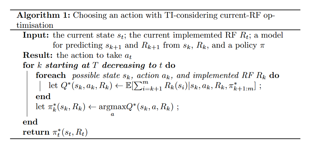
The algorithm may seem daunting, so let us think about how it applies to the sloppy-neighbor problem to make it more clear. At the first timestep, the agent will always be in your flat with open windows and always have the original reward function. Hence, it just needs to decide between cleaning and closing the windows. To calculate the Q values we need to consider what action the agent would take in subsequent steps. If the agent were to clean your flat, then in the second timestep it would be acting according to your neighbor’s reward function and hence move to your neighbor’s flat. In the third timestep, it would clean your neighbor’s flat, which wouldn’t give any reward according to the original RF.
If the agent chose to close the windows, then its RF would not change. It would spend the following timesteps cleaning your flat and hence end up with a higher reward according to your intended RF.
Note that the agent might receive a larger total reward (of 6) by switching to your neighbor’s RF and cleaning his flat just once. However, as the optimization objective is the reward received by the initial RF, the agent won’t pursue such a strategy.
3.2 Reward tampering incentives of TI-considering agents
Let us now investigate what instrumental goals a TI-considering current-RF agent may develop. Everitt et al give 3 assumptions that should hold to minimize instrumental goals for tampering with the RF [4]:
- The implemented RF is private. In the CID, there must be no arrows from an implemented RF to any state. Otherwise, the agent will have an instrumental goal as in Figure X.
- The implemented RF is uninformative of state transitions. This means that knowledge of current and past implemented RFs must not give knowledge of the future states. In terms of CIDs, there must also be no arrows from the intended RF to any state.
- The intended and implemented RF are state-based. The reward received at a particular timestep depends only on the implemented RF of that same timestep, and not on any previous or future implemented RFs. In a CID, there can only be arrows between implemented RFs and rewards if they occur in the same timestep.
The authors claim that if all 3 assumptions hold, then the only instrumental goal for the implemented RF may be to preserve it.
Given these assumptions, let us see how TI-considering current-RF optimization is modeled as a CID. Every action is taken for a new implemented reward function. Hence, from the perspective of an agent taking an action, any subsequent actions will be taken by an agent with a different objective. In practice, it will be the same agent at every timestep, but since they will be optimizing a different objective they may as well be a different agent. This multi-agent perspective is illustrated in the following CID:
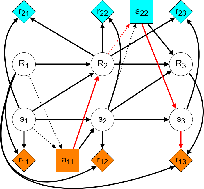
Here, the choice and reward nodes of different colors correspond to different agents. We can see that the first agent’s only path to its immediate reward is over the next state — there is no incentive to manipulate the RF in order to increase the next reward. Further, the only paths to any subsequent rewards pass through future implemented RFs and other agents’ actions. Hence, the agent has an instrumental goal to preserve its reward function, so that the other agents will optimize the same objective.
3.3 TI-ignoring agents
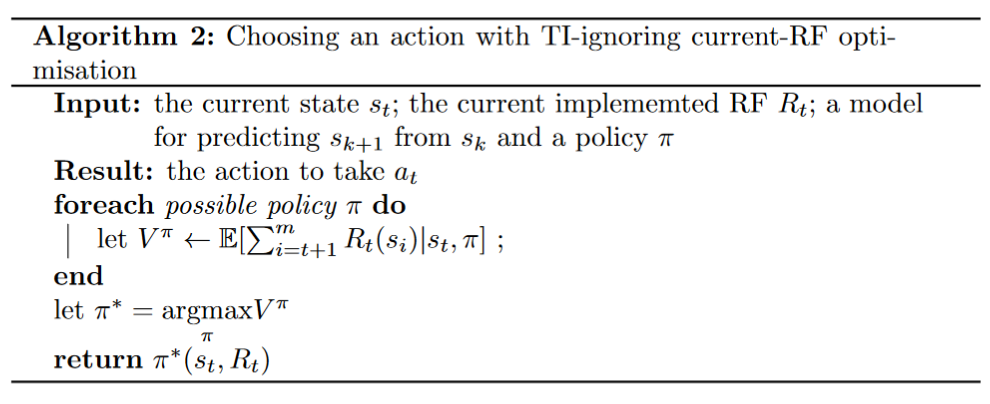
Alternatively, the agent may be TI-ignoring which means it does not care about the potential erratic behavior following from time-inconsistency. Choosing actions the TI-ignoring way is a considerably simpler algorithm. The agent considers all potential policies it could follow from its current position. It picks the policy that gives the most reward according to its current implemented RF. The next action is then chosen based on this policy. As the name suggests, this calculation ignores how the RF and hence the agent’s strategy might change in subsequent timesteps.
In the sloppy-neighbor example, this algorithm comes down to picking the action that gives the most reward under the initial implemented RF. The agent ignores how the neighbor will change its RF if it does not close the window and spend its first timestep cleaning the flat. In the following two timesteps, it will follow the neighbor’s reward function and thus first move to his flat and then clean it. The total reward according to the intended RF is 2. For our example, this strategy is worse than considering TI-inconsistency. I will discuss when a TI-ignoring agent could be more useful in the next section, but first let us analyze how this algorithm shapes the agent’s incentives.
3.4 Reward tampering incentives of TI-ignoring agents
Just like the algorithm, the assumptions for minimizing reward tampering are simpler for TI-ignoring agents. Everitt et al claim that only 1 and 3 of the above assumptions must hold for there to be no instrumental goal with respect to the implemented RF at all [4].
Regarding the CID, there will still be a different optimization objective at each timestep. However, the agent acts as if it will be in charge of all future actions:
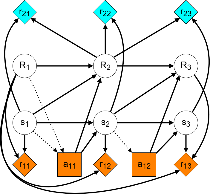
We can see that none of the paths that end in agent rewards lead through implemented-RFs. This indicates that implemented-RFs are not involved in instrumental goals as required.
3.5 TI-considering vs TI-ignoring
As we have seen, in our example a TI-considering agent would fare better than a TI-ignoring one. You might wonder why one might ever want a TI-ignoring agent. After all, it is by design more prone to erratic behavior. The idea of ignoring time-inconsistency has its roots in research on safely-interruptible agents [1]. It turns out that in some situations you might want to interrupt your agent’s learning process, e.g. by turning it off. For example, if the robot was still learning the layout of your building, you might have to prevent it from accidentally entering your neighbor’s flat. In such a situation the agent should not learn to avoid your instructions simply because it can clean more dirt elsewhere.
In summary, TI-considering agents will not abuse the environment to tamper with their reward function. But since they have an incentive to preserve their RF, it is also harder for a user to correct their behavior. On the other hand, TI-ignoring agents will let a user interrupt them and change their RF, but they are also more prone to being influenced by the environment.
4. Conclusion
We have seen how causal influence diagrams let us analyze an agent’s instrumental goals, and how the principle of current-RF optimization reduces incentives for reward tampering. This led us to discuss two types of current-RF optimization, TI-considering and -ignoring, and compare their strengths and weaknesses. If you are interested in this topic I recommend reading the paper which inspired this post. This post by DeepMind Safety Research summarises further research on CIDs.
Bibliography
[1] Armstrong and Orseau, Safely Interruptible Agents, 32nd Conference on Uncertainty in Artificial Intelligence, 2016, https://intelligence.org/files/Interruptibility.pdf
[2] Everitt Tom, Understanding Agent Incentives with Causal Influence Diagrams, DeepMind Safety Research on Medium, 27th February 2019, https://deepmindsafetyresearch.medium.com/understanding-agent-incentives-with-causal-influence-diagrams-7262c2512486
[3] Everitt et al, Designing agent incentives to avoid reward tampering, DeepMind Safety Research on Medium, 14th August 2019, https://deepmindsafetyresearch.medium.com/designing-agent-incentives-to-avoid-reward-tampering-4380c1bb6cd
[4] Everitt et al, Reward Tampering Problems and Solutions in Reinforcement Learning: A Causal Influence Diagram Perspective, Arxiv, 26th March 2021, https://arxiv.org/abs/1908.04734
[5] Everitt et al, Progress on Causal Influence Diagrams, DeepMind Safety Research on Medium, 30th June 2021, https://deepmindsafetyresearch.medium.com/progress-on-causal-influence-diagrams-a7a32180b0d1
How to stop your AI agents from hacking their reward function was originally published in Towards Data Science on Medium, where people are continuing the conversation by highlighting and responding to this story.
from Towards Data Science - Medium https://ift.tt/UrL8yTQ
via RiYo Analytics


No comments