https://ift.tt/B6a8UVf Using RNNs for Sentiment Analysis Photo by Nishaan Ahmed from Unsplash This article will discuss a separate se...
Using RNNs for Sentiment Analysis

This article will discuss a separate set of networks known as Recurrent Neural Networks(RNNs) built to solve sequence or time series problems.
Let’s dive right in!
What is a Recurrent Neural Network?
A Recurrent Neural Network is a special category of neural networks that allows information to flow in both directions. An RNN has short-term memory that enables it to factor previous input when producing output. The short-term memory allows the network to retain past information and, hence, uncover relationships between data points that are far from each other. RNNs are great for handling time series and sequence data such as audio and text.
RNN Structure
The image below shows the structure of the RNN.
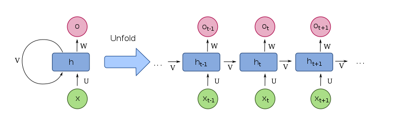
The unrolled network results from creating a copy of the RNN for every time step t. ht denotes the output of the network at time t, while Xt is the input to the network at time t.
Types of RNNs
Let’s now briefly mention various types of RNNs.
There are four main types of RNNS:
- One to one that has a single input and a single output.
- One to many with a single input and multiple outputs, for example, image captioning.
- Many to one with multiple inputs and a single output, for example, sentiment analysis.
- Many to many with many inputs and many outputs, for example, machine translation.
How does a Recurrent Neural Network work?
As you can see in the above unrolled RNN, RNNs work by applying backpropagation through time (BPPTT). In this manner, weights for the current and previous input are updated. The weights are updated by propagating the error from the last to the first time step. As a result, the error for each time step is computed.
RNNs are not able to handle long-term dependencies. Two major problems arise in very long time steps: vanishing gradients and exploding gradients.
RNN challenges — The vanishing gradient problem
Vanishing gradients occur when the gradients used for computing the weights start vanishing, meaning that they become small numbers close to zero. As a result, the network doesn’t learn. The opposite of this is the exploding gradients problem.
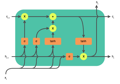
The exploding gradient problem is solved by clipping the gradients. The vanishing gradient problem is fixed by a certain type of RNNs that can handle long-term dependencies, for example, Long Short-Term Memory(LSTMs).
LSTMs
There are several variations of Recurrent Neural Networks. Here are a couple of them:
- Long Short Term Memory (LSTM) solves the vanishing gradient problem by introducing input, output, and forget gates. These gates control which information is retained throughout the network.
- Gated Recurrent Units (GRU) that handle the vanishing gradient problem by introducing reset and updated gates that determine which information is retained throughout the network.
In this tutorial, our primary focus will be on LSTMs. LSTMs can handle long-term dependencies and are more suited for problems with long sequences such as sentiment analysis. For example, in a long movie review, it’s important to remember the beginning of the review in deciding the review’s sentiment. Consider the review, “The movie was quite slow and some characters were quite boring, but overall, it was a very interesting movie.” If you only consider the first part of this review, you’d label it as a negative review. However, towards the end of the review, the viewer says that the movie was interesting.
Implementing LSTMs for sentiment analysis
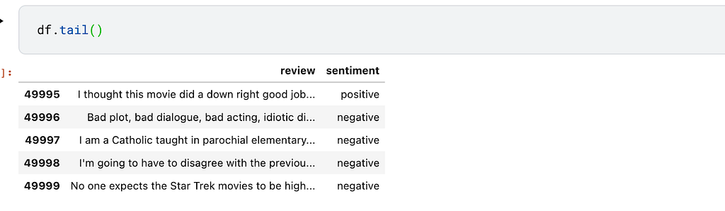
Next, let’s implement LSTM for sentiment analysis in TensorFlow. We’ll use the famous IMDB Dataset of 50K Movie Reviews dataset that’s available on Kaggle. The dataset is publicly available on the Stanford website.
We’ll use Layer to fetch the data as well as run the project. The first step, therefore, is to authenticate a Layer account and initialize a project.
The get_dataset function can be used to obtain the dataset.
Next, let’s define a function to remove common words from the reviews.
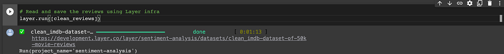
Let’s now use the above function to clean the reviews. We can save the cleaned dataset so that we don’t repeat this process again.
Saving the dataset to Layer is done by decorating the function with the @dataset decorator. The pip_requirements decorator is used to pass in the packages required to run this function.
Executing the above function will save the data and output a link that can be used to view it.
Text preprocessing
Since the data is in text form, we need to convert it into a numerical representation. Furthermore, we have to do the following:
- Remove special characters and punctuation marks.
- Convert the reviews to lowercase.
We can perform all the above operations using the Tokenizer class from TensorFlow. This is done by creating an instance of the class and fitting its fit_on_texts method on the training set. While doing so, we define an out-of-vocabulary token that will be used for replacing out-of-vocabulary words when converting the text to sequences later. By default the tokenizer will keep the most common words, however, this can be overridden using the num_words argument.
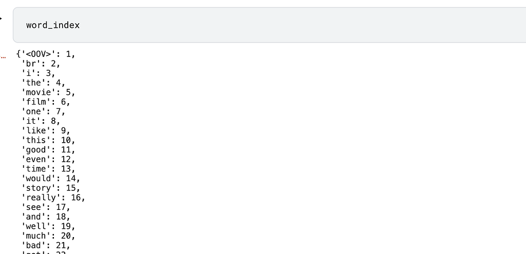
At this point, each word is now mapped to an integer representation. This is known as the word index and can be seen by calling the word_index on the tokenizer.
It would be lovely if we can save this tokenizer so that we don’t have to train the tokenizer on this dataset again. Let’s create a function to save this tokenizer. We use the @model decorator because the function returns a model. The @fabric decorator dictates the type of environment where the function will be executed.
Executing the above function will train the tokenizer and save it.
Create text sequences
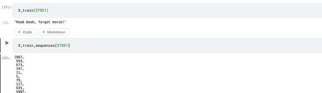
Now that each word has an integer representation, we need to create a sequence representation for each review. This is done by the texts_to_sequences function. We fetch the tokenizer we just saved and use it for this operation.
Here’s an image showing a review and its numerical representation:
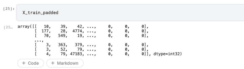
Pad the text sequences
One of the challenges of working with these reviews is that they are of different lengths. However, the LSTM neural network we’ll build in a moment expects the data to be of the same length. We solve this by defining a maximum length for each review and truncating them. After that, we pad reviews below the maximum length with zeros. The padding can be done at the beginning (pre) or the end of the review (post). pad_sequences is a preprocessing method obtained from TensorFlow.
Here is how the data looks like after padding:
Before creating the LSTM model let’s bundle the data into a TensorFlow dataset.
Define the LSTM model
With the data ready, we can create a simple LSTM network. We’ll use the Keras sequential API for that. The network will consist of the following major building blocks:
- An Embedding Layer. A word embedding is a representation of words in a dense vector space. In that space words that are semantically similar appear together. For instance, this can help in sentiment classification in that negative words can be bundled together.
The Keras embedding Layer expects us to pass the size of the vocabulary, the size of the dense embedding, and the length of the input sequences. This layer also loads pre-trained word embedding weights in transfer learning.
- Bidirectional LSTMs allow data to pass from both sides, that is from left to right and from right to left. The output from both directions is concatenated but there is the option to sum, average, or multiply. Bidirectional LSTMs help the network to learn the relationship between past and future words.
When two LSTMs are defined as shown below, the first one has to return sequences that will be passed to the next LSTM.
Let’s now bundle the above operations into a single training function. The function will return the LSTM model. To save this model, its metrics, and parameters, we wrap it with the @model decorator.
Executing the above function trains and saves the model. it also logs all the items defined in the function such as the training and validation accuracy.

The trained model is now ready for making predictions on new data.
Final thoughts
In this article, we have talked about the Recurrent Neural Network and its variations. Specially, we have covered:
- What is a Recurrent Neural Network?.
- The structure of a Recurrent Neural Network.
- Challenges of working with RNNs.
- How to implement an LSTM in TensorFlow.
Images used with permission.
Dataset citation
@InProceedings{maas-EtAl:2011:ACL-HLT2011,
  author    = {Maas, Andrew L.  and  Daly, Raymond E.  and  Pham, Peter T.  and  Huang, Dan  and  Ng, Andrew Y.  and  Potts, Christopher},
  title     = {Learning Word Vectors for Sentiment Analysis},
  booktitle = {Proceedings of the 49th Annual Meeting of the Association for Computational Linguistics: Human Language Technologies},
  month     = {June},
  year      = {2011},
  address   = {Portland, Oregon, USA},
  publisher = {Association for Computational Linguistics},
  pages     = {142--150},
  url       = {http://www.aclweb.org/anthology/P11-1015}
}
Getting Started with Recurrent Neural Network (RNNs) was originally published in Towards Data Science on Medium, where people are continuing the conversation by highlighting and responding to this story.
from Towards Data Science - Medium https://ift.tt/X5BrLEI
via RiYo Analytics


ليست هناك تعليقات