https://ift.tt/m5WX6E8 Image from Pixabay A comprehensive read on support vector classification Machine learning opens a lot of possib...

A comprehensive read on support vector classification
Machine learning opens a lot of possibilities when it comes to identifying and solving specific problems in your field. Trying to master Machine Learning can be both complex and difficult to understand at times. Most beginners start by learning regression for its simplicity and ease, yet that doesn’t solve our purpose! One can do so much more than just regression when it comes to using different types of algorithms for different applications.
Classification is one such field of application for various supervised learning algorithms. With the exception of unnatural trends and momentum, often these classifiers have similar performance. However, when it comes to the complexity of the data and its scope, Support Vector Machines can be a good choice to articulate better decisions.
Before continuing with this article, I would suggest you do a quick read-through of my previous articles — A Quick and Dirty Guide to Random Forest Regression, and Unlocking the True Power of Support Vector Regression to swot upon the concepts of Ensemble Learning and SVMs. If you find this article informative, do consider clapping for this article so that it reaches more people, and follow me for more #MachineLearningRecipes.
Support Vector Machine Under the Hood
Everything that happens in Machine Learning has a direct or indirect mathematical intuition associated with it. Similarly, with Support Vector Machines, there’s plenty of mathematics in the sea. There are various concepts such as length and direction of the vector, vector dot product, and linear separability that concern the algorithm.
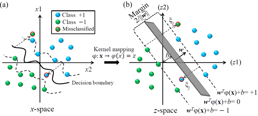
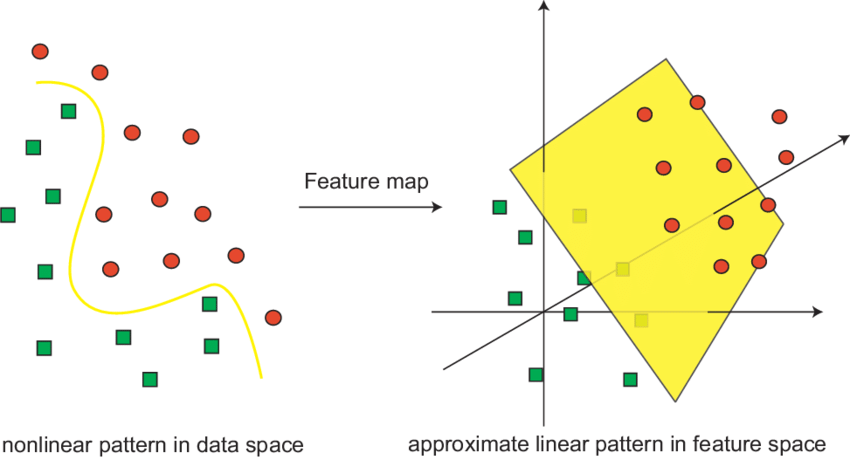
While this is an important part of the study, it is mostly studied by researchers, trying to optimize and/or scale the algorithm. In this section, we will only look into the mathematical intuition behind defining the hyperplane and the classifier. The two-dimensional linearly separable data can be separated by a line. The function of a straight line is given by y=ax+b. On renaming x with x1 and y with x2, we get ax1−x2+b=0.
If we define x = (x1,x2) and w = (a,−1), we get: w⋅x+b=0. This is the equation of the hyperplane. Once the hyperplane has been defined, it can then be used to make predictions. The hypothesis function h. The point above or on the hyperplane will be classified as class +1, and the point below the hyperplane will be classified as class -1.
What are Support Vector Machines?
Support Vector Machines or SVMs have supervised learning algorithms that can be used with both regression and classification tasks. Owing to its robustness, it’s generally implemented for solving classification tasks. In this algorithm, the data points are first represented in an n-dimensional space. The algorithm then uses statistical approaches to find the best line that separates the various classes present in the data.

If the data points are plotted in a 2-dimensional graph, then the decision boundary is referred to as a straight line. However, if there are more than two dimensions, these are referred to as hyperplanes. While there may be multiple hyperplanes that separate the classes, SVM chooses the one with the maximum distance between the classes.
This distance between the hyperplane and the closest data points(called support vectors) is referred to as Margin. Margin may be either soft margin or, hard margin. When data can be separated into two distinct sets, and we don’t want to have any misclassifications, we use our training set weights during crossover to train the SVMs with a hard margin.
However when we need more generality out of our classifier, or when the data cannot be cleanly divided into two distinct groups, we should opt for a soft margin in order to allow some non-zero misclassification. SVMs are generally used with small, and robust datasets that are usually complex.
SVMs without kernels may have similar performance as that of logistics regression algorithm, and can thus be used interchangeably. Unlike the logistic regression algorithm which considers all data points, the support vector classifier only considers the data points closest to the hyperplane i.e. the Support Vectors.
SVM Classification Libraries
Scikit-learn contains many useful libraries to implement SVM algorithms on a set of data. There are several libraries we have at our disposal that can help us when it comes down to implementing Support Vector Machine smoothly. This is mainly due to the fact that these libraries pose all of the necessary functions we need in order to apply SVM without too much hassle on our part.
First, there is a LinearSVC() classifier. As the name suggests, this classifier uses only a linear kernel. In LinearSVC() classifier, we don’t pass the value of the kernel since it is used only for linear classification purposes. Scikit-Learn provides two other classifiers — SVC() and NuSVC() which are used for classification purposes.
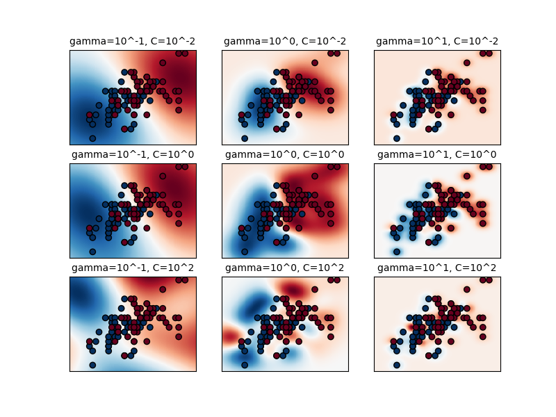
These classifiers are mostly similar with some differences in parameters. NuSVC() is similar to SVC() but uses a parameter to control the number of support vectors. Now that you have a crux of what support vector classification is, we shall try to build our very own support vector classifier. The code and other resources for building this regression model can be found here.
Step 1: Importing the Libraries and Fetching the Dataset:
In the first step, import the libraries that we will be using for implementing the SVM classifier in this example. It is not necessary to import all the libraries in just one place. Python gives us the flexibility to import libraries at any place. To get started we will be importing the Pandas, Numpy, Matplotlib, and Seaborn libraries.
import numpy as np
import pandas as pd
import matplotlib.pyplot as plt
import seaborn as sns
%matplotlib inline

import os
for dirname, _, filenames in os.walk('/kaggle/input'):
    for filename in filenames:
        print(os.path.join(dirname, filename))
For this example the Predicting a Pulsar Star dataset has been used. This data set contains 16,259 spurious examples caused by RFI/noise and 1,639 real pulsar examples. Each row lists the variables first, and the class label is the final entry. The class labels used are 0 (negative) and 1 (positive).
Step 2: Exploratory Data Analysis and Visualization:
After successfully loading the data, our next step is to explore the data to gain insights about the data. There are 9 variables in the dataset. 8 are continuous variables and 1 is a discrete variable. The discrete variable is the target_class variable. It is also the target variable.
df.columns = ['IP Mean', 'IP Sd', 'IP Kurtosis', 'IP Skewness',
              'DM-SNR Mean', 'DM-SNR Sd', 'DM-SNR Kurtosis', 'DM-SNR Skewness', 'target_class']
df.column
df['target_class'].value_counts()/np.float(len(df))
df.info()
plt.figure(figsize=(24,20))
plt.subplot(4, 2, 1)
fig = df.boxplot(column='IP Mean')
fig.set_title('')
fig.set_ylabel('IP Mean')
Renaming the columns, removing the leading spaces, and dealing with the missing values are also part of this step. After cleaning the data, the data set is visualized to understand the trend. Seashore is an excellent library that can be used to visualize the data.
Step 3: Feature Engineering and Fitting the Model:
Feature engineering is the process of using domain knowledge to extract features from raw data via data mining techniques. For this model, I have selected columns with only numerical values.
For handling categorical values label encoding techniques are applied. Default hyperparameter means C=1.0, kernel=rbf, and gamma=auto among other parameters.
from sklearn.preprocessing import StandardScaler
scaler = StandardScaler()
X_train = scaler.fit_transform(X_train)
X_test = scaler.transform(X_test)
After selecting the desired parameters the next step is to import train_test_split from sklearn library which is used to split the dataset into training and testing data. After this SVR is imported from sklearn.svm and the model is fit over the training dataset.
Step 4: Accuracy, Precision, and Confusion Matrix:
The classifier needs to be checked for overfitting and underfitting. The training-set accuracy score is 0.9783 while the test-set accuracy is 0.9830. These two values are quite comparable. So, there is no question of overfitting. Precision can be defined as the percentage of correctly predicted positive outcomes out of all the predicted positive outcomes.
It can be given as the ratio of true positives (TP) to the sum of true and false positives (TP + FP). A confusion matrix is a tool for summarizing the performance of a classification algorithm. A confusion matrix will give a clear picture of classification model performance and the types of errors produced by the model.
It gives a summary of correct and incorrect predictions broken down by each category. This summary is represented in a tabular form. A classification report is another way to evaluate the classification model performance. It displays the precision, recall, f1, and support scores for the model
svc=SVC()
svc.fit(X_train,y_train)
y_pred=svc.predict(X_test)
print('Model accuracy score with default hyperparameters: {0:0.4f}'. format(accuracy_score(y_test, y_pred))
Another tool to measure the classification model performance visually is ROC Curve. ROC Curve stands for Receiver Operating Characteristic Curve. A ROC curve is a plot that shows the performance of a classification model at various classification threshold levels.
Advantages of SVM Classifier:
Support Vector Classification carries certain advantages that are as mentioned below:
- SVM works relatively well when there is a clear margin of separation between classes.
- SVM is more effective in high dimensional spaces and is relatively memory efficient
- SVM is effective in cases where the dimensions are greater than the number of samples.

Disadvantages of SVM Classifier:
Some of the drawbacks faced by SVM while handling classification is as mentioned below:
- SVM algorithm is not suitable for large data sets.
- SVM does not perform very well when the data set has more noise i.e. target classes are overlapping. In cases where the number of features for each data point exceeds the number of training data samples, the SVM will underperform.
- As the support vector classifier works by putting data points, above and below the classifying hyperplane there is no probabilistic explanation for the classification.
With that, we have reached the end of this article. I hope this article would have helped you get a feel about the idea behind SVC algorithms. If you have any questions or if you believe I have made any mistakes, please contact me! You can get in touch with me via Email or LinkedIn.
Everything About Support Vector Classification — Above and Beyond was originally published in Towards Data Science on Medium, where people are continuing the conversation by highlighting and responding to this story.
from Towards Data Science - Medium https://ift.tt/cza6hS9
via RiYo Analytics

No comments