https://ift.tt/ojp5cVk Upgrade Variance Reduction Beyond CUPED: Introducing MLRATE MLRATE uses machine learning to reach statistical power...
Upgrade Variance Reduction Beyond CUPED: Introducing MLRATE
MLRATE uses machine learning to reach statistical power more quickly when experimenting.
Say you are running an experiment, and there is a true difference in the means between your control and variant population. Will you detect it? That depends on three things:
- The size of the effect
- The number of your samples you collect
- The variance of your measurement
The size of your effect isn’t often something you can alter. Increasing sample size takes more time and can be costly too. So we are left staring at option three: how can we make our measurement less noisy?
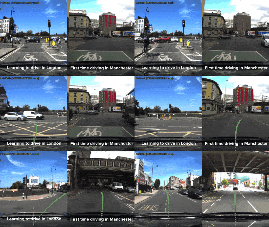
At Wayve we are developing autonomous driving technology using end-to-end deep learning, so evaluating the difference in real-world driving performance between two models on the road in both the quickest and most robust way is very important. One challenge is that conditions vary notably between runs: from weather to traffic density to jay-walking pedestrians. So, rather than treat differing conditions as noise that averages out when experimenting (as per traditional experiment procedures), we instead want to use the signal and learn from every interaction.
Using a machine-learning-adjusted treatment effect estimator (MLRATE, Meta 2022) we can exploit the complex non-linear relationships that machine learning models can learn between such confounding variables and driving performance, and implement this in a robust way using a generalized linear model. This allows us to reach statistical significance with a smaller sample size. For example, at Wayve, we have found we can half the number of driven km we need to reach statistical significance using MLRATE.
Some context: simple A/B tests can be highly inefficient
Randomised controlled tests (RCTs) are traditionally the gold standard to measure improvements. RCTs are often used in the tech industry to test machine learning models online, typically randomly splitting a user base into a control group (users treated with the old ML model) and variant group (users treated with the new ML model), and observing the difference in the means of a performance metric between the two groups (an A/B test, deriving the ‘difference-in-means estimator’). These experiments often capture millions of data points for this process: the large scale randomization is important to ensure we have a representative sample for testing, to facilitate fairer comparisons, and to give greater statistical confidence that a measured improvement is genuine rather than just noise.
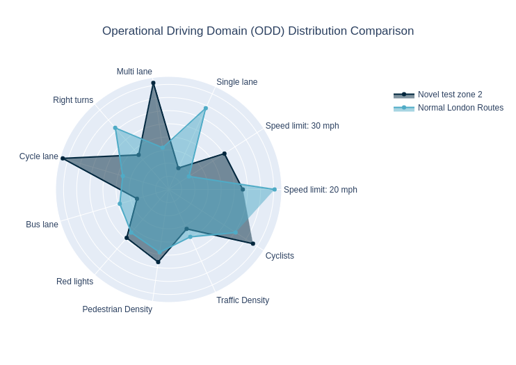
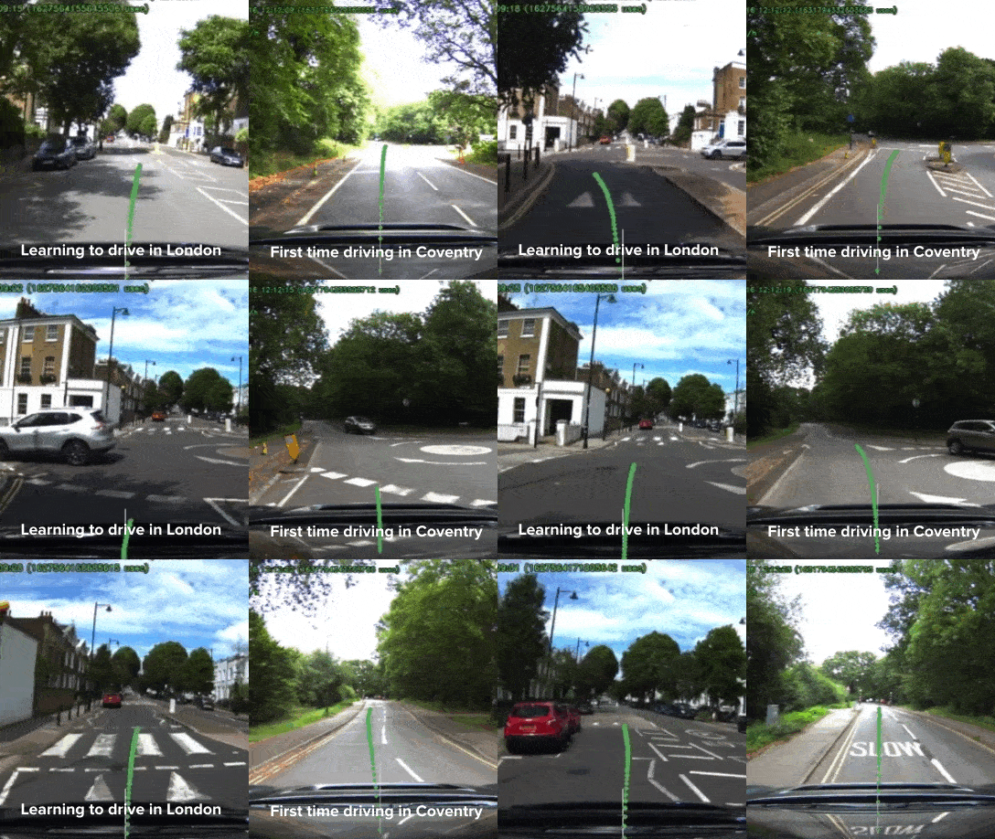
But large-scale randomisation doesn’t work for real-world driving. Randomly testing routes means huge differences in the scenery a driving model has to navigate, from traffic islands to construction zones — this variance would make us uncertain in our conclusions without a huge sample size, and it is not feasible to collect so much driving data for every new model when we want to iterate and learn quickly. Even testing two driving models on the same route (i.e. paired tests) doesn’t solve for this. For example, we cannot control for dynamic agents such as cars or cyclists, or if one driving model has all green lights and the other one has all red lights instead. Further, restricting to specific routes could mean over-optimizing for these specific test routes. Wayve wants to be the first company to reach 100 cities autonomously: we can’t just tailor our testing to the roads we drive today, and we need to compare driving models that haven’t driven on the same segments of road, utilising an understanding of how well our cars perform in areas they have never even driven before.
Typical variance reduction techniques can attain statistical significance faster, but we can go further
Data scientists often employ variance-reduction techniques to improve detection of genuine improvements that would be too small to parse with statistical confidence at a lower sample size. For example, one might find drivers are most performant at roundabouts when traffic density is lower. Measuring roundabout performance of a driver, across all levels of traffic, would have a larger variance in measurement — so we would be less sure if an observed performance difference is genuine or due to chance. We expect that when one driver faces less traffic they would perform better, so we should incorporate this pre-existing knowledge into our experiment.
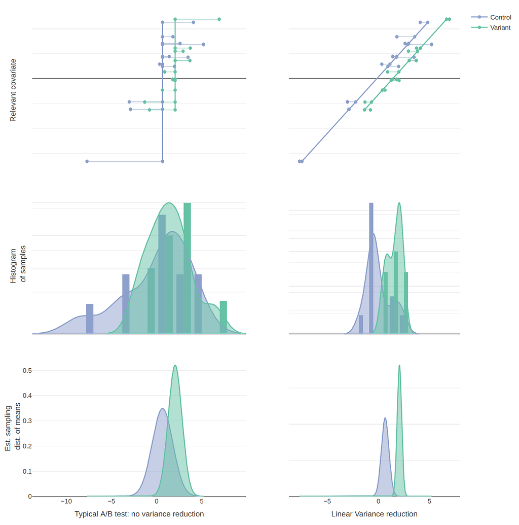
A common method used for variance-reduction is through Controlled-experiments Using Pre-Existing Data (CUPED, Microsoft 2013), where some linear covariates (such as traffic density) are used to adjust the simple difference-in-means estimator.
This is essentially equivalent to simple linear regression! Which is useful to denote now to best contextualise MLRATE later on:

Where:
- Y is a vector of the measured values for each observed sample
- V is a dummy variable recording whether the collected sample was in the variant group or not
- X record the value of the relevant covariate when that sample was collected
Hence, we care about estimating the coefficient 𝛿1 (the size of the improvement in our metric y due to being in the variant group instead of the control). Including a simple dummy variable v effectively de-means each sample by the group mean, so this is equivalent to usual t-tests.
The resultant standard error for 𝛿1 is larger when omitting the relevant variable x as can seen in the graphs on the left above — including it reduces the standard error and hence it is more likely to be statistically significant. In general, the more highly correlated the covariate is with y, the more the variance is reduced.
(Note, there is no expected bias from omitted relevant variables in this regime, as we assume the allocation of a sample to treatment or control, v, is independent of x i.e. they are orthogonal).

However, whilst CUPED is highly effective at variance reduction for a few variables that are linearly related, adjusting for many covariates with complex non-linear relationships is often not in scope.
At Wayve, we want to incorporate many confounding variables into our testing that affect performance, such as static scenery differences (e.g. bus lanes, pedestrian crossings), dynamic agents (traffic density, presence of cyclists), environmental factors (e.g. weather, luminosity) and even human biases from safety operations(and these often have complex non-linear interactions between them too). Using a more complex machine learning model would provide a more sophisticated proxy to facilitate controls for these covariates.
MLRATE follows two steps to reduce variance using ML models in a robust way
Step 1: Train and calibrate an ML model
To control for all desired covariates, the first step involves building a machine-learning model to predict our performance metric using relevant covariates.
At Wayve we train an artificial neural network (multi-layer perceptron) on a balanced dataset, using all the features we are interested in controlling for during testing (such as dynamic agents). ANNs tend to be overconfident in their prediction, so we also calibrate using isotonic regression to ensure our performance predictions are linearly related with actual performance (this is important for the second step, that we will allude to later).
For this first step in practice, we randomly split our training data in two: we train and calibrate two performance-prediction models with the same architecture, one on each dataset, then predict performance for each sample in each dataset using the model it wasn’t trained on. This method of ‘cross-fitting’ (using out-of-sample prediction) is important to avoid attenuation biases that could result from over-fitting if in-sample predictions were used instead.
Step 2: Estimate the ML-adjusted treatment effect using GLM
For the second step, we model the actual performance as a function of the predicted control performance using a generalised linear model. This ensures our testing is robust even if the ML prediction is poor. In fact, regardless of how bad the outcome predictions from the performance-prediction step are, MLRATE has an asymptotic variance no larger than the usual difference-in-means estimator: in other words, MLRATE benefits if the machine learning predictions from the previous step are good, but robust to increased variance if the predictions are poor.
Similar to before, this step involves running a generalized linear model, but instead of using x (a linear covariate), g(X) is used to show how we incorporate predictions from the ML step.

In addition to the previous regressions, an interaction term between the treatment and the prediction is used to account for the fact than the prediction term might be less correlated — and thus result in omitted relevant bias on d_1. (Note these values are de-meaned to prevent high multi-collinearity with our dummy variable, which could otherwise make that coefficient erratic).
The MLRATE paper uses Huber-White heteroskedasticity-corrected standard errors to derive the confidence interval for this estimator (which determines whether the coefficient is statistically significant). However, we often use more-conservative clustered standard errors due to the experimental setups we have at Wayve.
Tailoring comparisons using weights
At Wayve, we take the MLRATE methodology a step further, tailoring our model evaluation to enable comparisons that better suit the specific ODD attributes of routes. For example, our models may have been tested mainly on 20mph, high traffic density roads, but on the typical route of a grocery partner we have more 30mph, multi-lane roads with lower traffic density. We thus might want to weight our 30mph, multi-lane scenarios more highly, and do so accordingly to match this target distribution, rather than run the regression as if each trial is equally important.

We take inspiration from running generalized linear models on survey data, typically conducted by decision scientists, to achieve this. We create weights for every trial (analogous to design weights in survey data) using features we know are predictive of performance, and run weighted regressions instead.
Traditionally, iterative proportional fitting is used to define weights to ensure the marginal totals are the same. However, using IPF means the joint distribution of the features we care about can be quite different from the target. So although IPF was explored, Wayve intentionally chooses not to do this, since we know the target joint distribution of our features of interest and we care about matching this joint distribution closely (particularly since some features are not independent and their co-occurence may have multiplicative impacts on performance). Instead, we derive weights to match the joint distribution of the features.
Weights are truncated to ensure rarely tested (potentially noisy) combinations of features do not have too high a weight (which we have determined by bootstrapping our testing data offline). The weights are also normalized to ensure the degrees of freedom in the regression step are the same as non-weighted GLM.
Automating this analysis
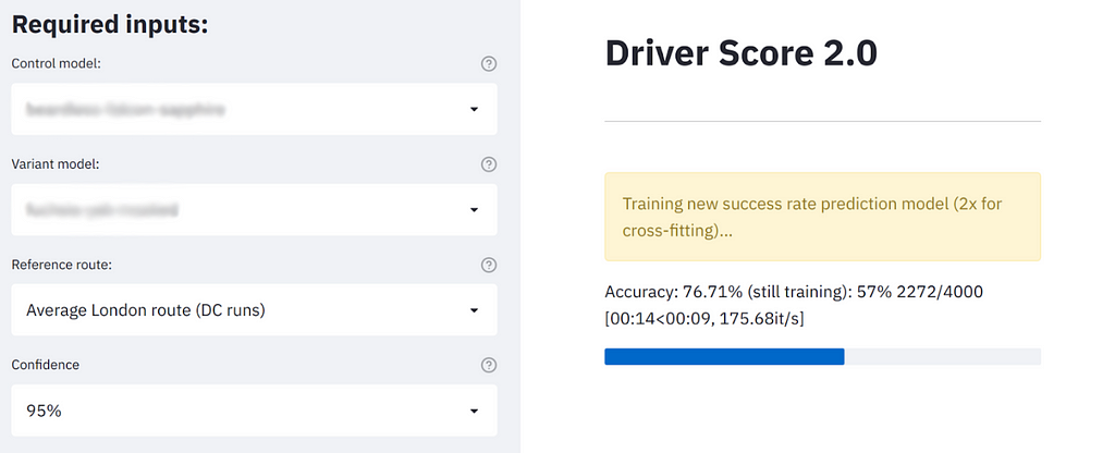
At Wayve, we have automated all of this analysis in our internal applications. ML researchers can provide specific filters and the routes they wish to tailor for before we automatically train neural networks and run generalised linear model on-the-fly, producing detailed reports in minutes. These tools facilitate rapid and robust comparisons between any two models, allowing us to accelerate our fleet learning loop and pack it full of insight derived across all the features we capture. We will publish a blog post shortly on this!
References and further reading:
- Robust Experiment Design
- Machine Learning for Variance Reduction in Online Experiments
- [PDF] Improving the sensitivity of online controlled experiments by utilizing pre-experiment data | Semantic Scholar
- Iterative proportional fitting - Wikipedia
- Analysis of Complex Survey Samples by Thomas Lumley
- Improving the Sensitivity of Online Controlled Experiments: Case Studies at Netflix
Variance reduction on steroids… introducing MLRATE was originally published in Towards Data Science on Medium, where people are continuing the conversation by highlighting and responding to this story.
from Towards Data Science - Medium https://ift.tt/prwFgTV
via RiYo Analytics

No comments