https://ift.tt/9fBCVN3 Semantic Segmentation of Aerial Imagery Using U-Net in Python Semantic Segmentation of MBRSC Aerial Imagery of Duba...
Semantic Segmentation of Aerial Imagery Using U-Net in Python
Semantic Segmentation of MBRSC Aerial Imagery of Dubai Using a TensorFlow U-Net Model in Python
This article aims to demonstrate how to semantically segment aerial imagery using a U-Net model defined in TensorFlow.

Introduction
Image Segmentation is the task of classifying an image at the pixel level.
Every digital picture consists of pixel values, and semantic segmentation involves labelling each pixel.
Dataset
The MBRSC dataset exists under the CC0 license, available to download. It consists of aerial imagery of Dubai obtained by MBRSC satellites and annotated with pixel-wise semantic segmentation in 6 classes. There are three main challenges associated with the dataset:
- Class colours are in hex, whilst the mask images are in RGB.
- The total volume of the dataset is 72 images grouped into six larger tiles. Seventy-two images is a relatively small dataset for training a neural network.
- Each tile has images of different heights and widths, and some pictures within the same tiles are variable in size. The neural network model expects inputs with equal spatial dimensions.
Figure 1 depicts a training set input image and its corresponding mask with superimposed class annotations.
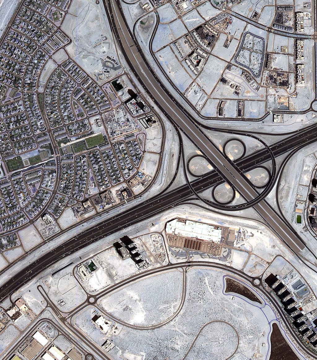
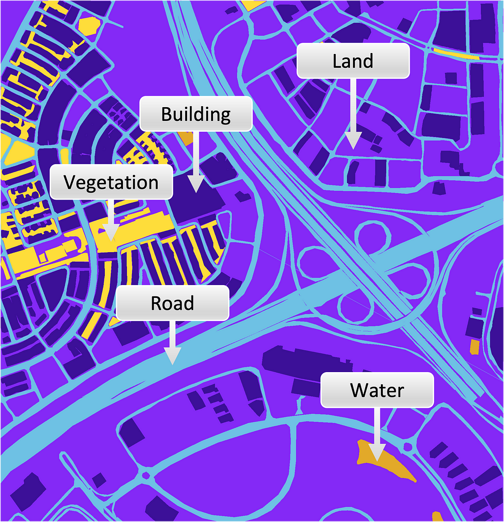
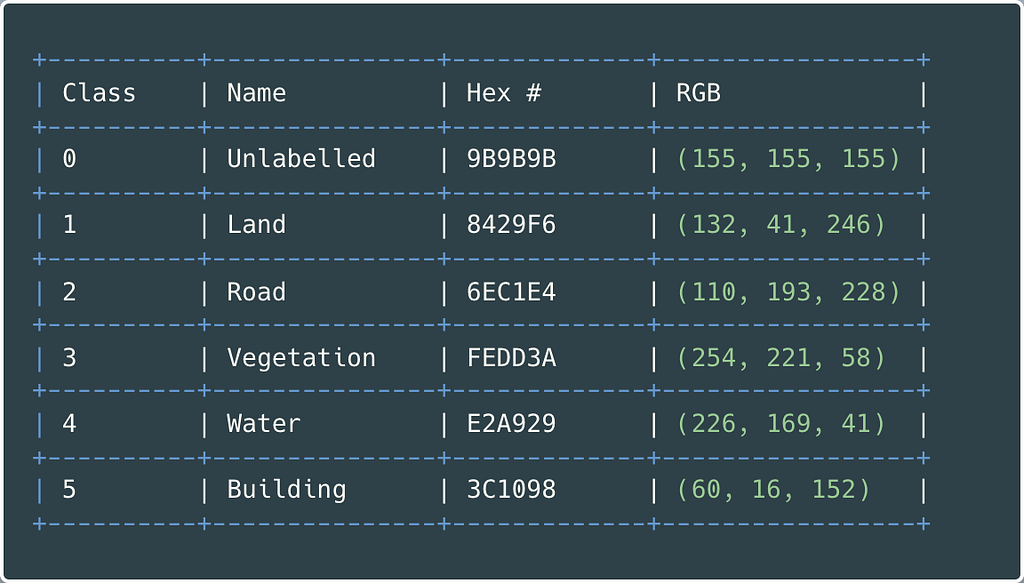
Table 1 presents each class name, corresponding hex colour code, and converted RBG values.
Preprocessing
Images must be the same size when fed into the neural network’s input layer. Therefore, before model training, images are decomposed into patches.
The patch_size chosen is 160 px. There is no ideal patch size; it serves as a hyperparameter that can be experimented with for performance optimisation.
Taking an image from Tile 7 with a width of 1817 pixels and a height of 2061 pixels, Expression 1 illustrates how to calculate the number of created patches.

Next, the images are cropped to the nearest size divisible by the patch_size to avoid patches with overlapping areas. Expression 2 determines the new trimmed width and height for the Tile 7 image.

Figure 2 clarifies the cropping and patching processes for a single image.
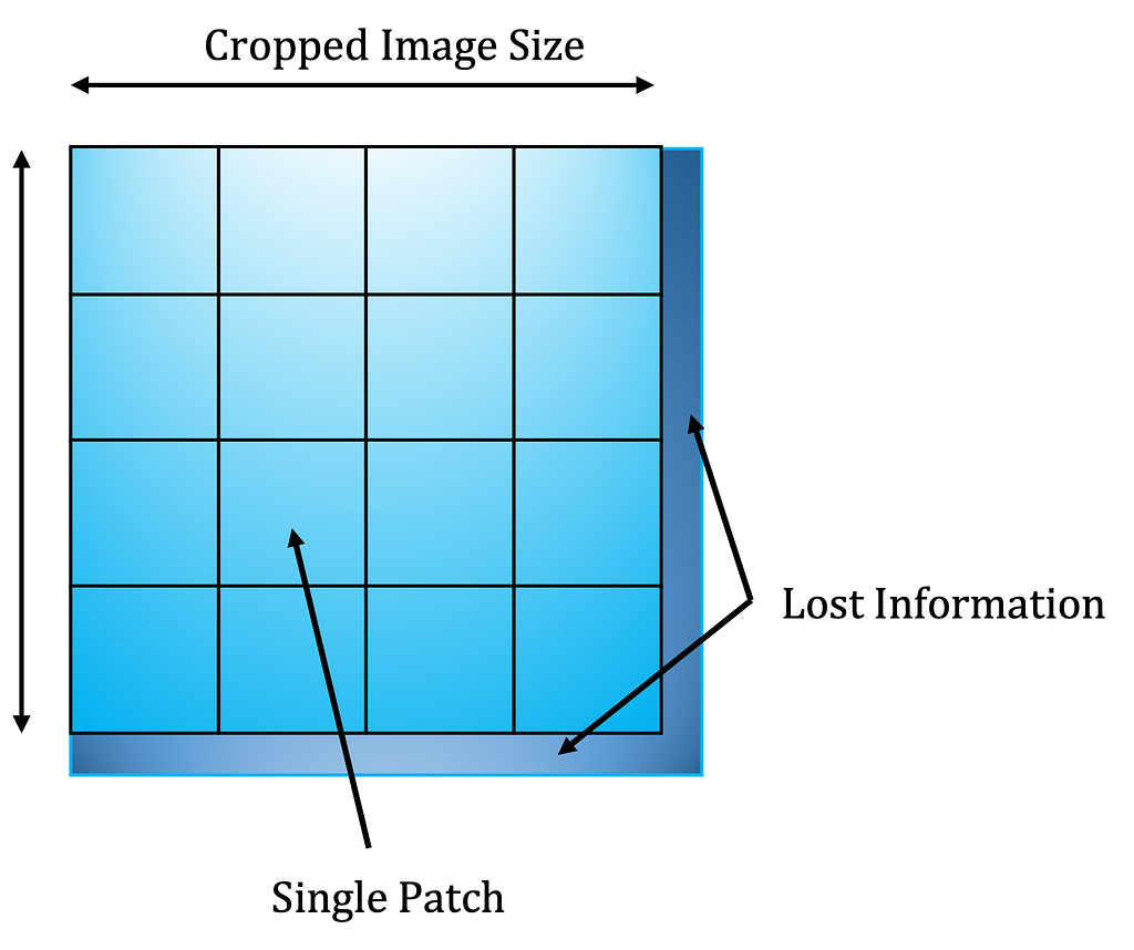
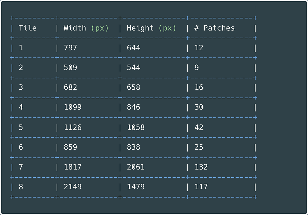
Table 2 gives tiles; their sizes are the total number of patches created using a size of 160 px.
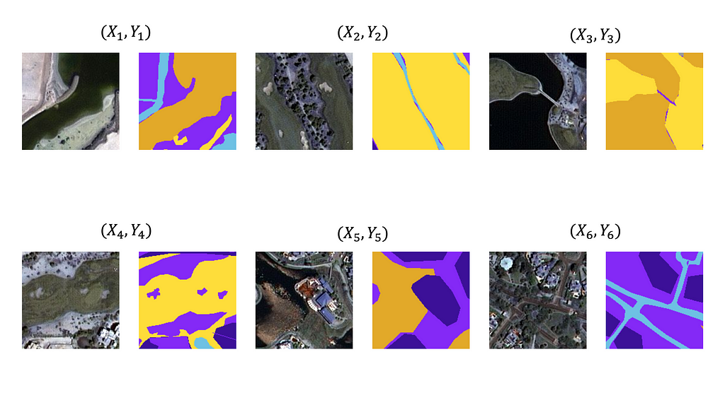
After cropping and patchifying, 3483 images and masks comprise the input dataset. Figure 3 presents six randomly selected image patches with their comparable mask.
Use the Python code from Gist 1 to load image files from a directory and perform the data preprocessing as described above.
The masks are tensors of shape (160, 160, 3). Axis 3, or the third dimension, is interpretable as a NumPy array of 8-bit unsigned integers. These range in value from 0 through 255, corresponding to the RGB colours listed in Table 2.
Multi-class classification problems require the outputs encoded as integers. i.e. for a Building class with RGB values (60, 16, 152), the appropriate label is 0.
To transform the third dimension of the mask into a one-hot encoded vector representing the appropriate class label, execute the Python code from Gist 2.
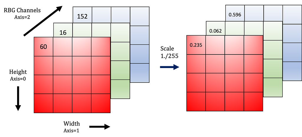
Currently, the input images are tensors interpretable as NumPy arrays of 8-bit unsigned integers (0 through 255 decimal). Therefore, rescaling the values from 0–255 to 0–1 improves performance and training stability.
Keras offers a Rescaling preprocessing layer, which modifies the input values to a new range. Define this layer using the Python code below.
rescaling_layer = layers.experimental.preprocessing.Rescaling(
    scale=1. / 255,
    input_shape=(img_height, img_width, 3)
)
Every input image value is multiplied by scale, as shown in Figure 4.
Generally, three sections are partitioned, training, validation and testing. However, the dataset is relatively small compared to other machine learning computer vision datasets. As a result, only a single split is necessary, and the inferences occur on the X_test dataset.
- X_train and Y_train consist of 90% of the training set
- X_test and Y_test make up the remaining 10% of the data
Model Architecture
Many pre-trained or pre-defined convolutional neural network (CNN) architectures exist for image segmentation tasks, for example, U-Net, which demonstrates superior ability in this area.
U-Net consists of two critical paths:
- Contraction corresponds to general convolution Conv2D operations, where filters slide across the input image extracting features.
Following Conv2D, the MaxPooling2D layer operates on groups of pixels and filters values by selecting the maximum. Pooling downsamples the input image size while maintaining feature information. - Expansion: the downsampled image expands using transpose convolutions or deconvolutions, Conv2DTranspose, to recover the input image spatial information. While upsampling, skip connections concatenate the features between the symmetric contraction and expansion layers.
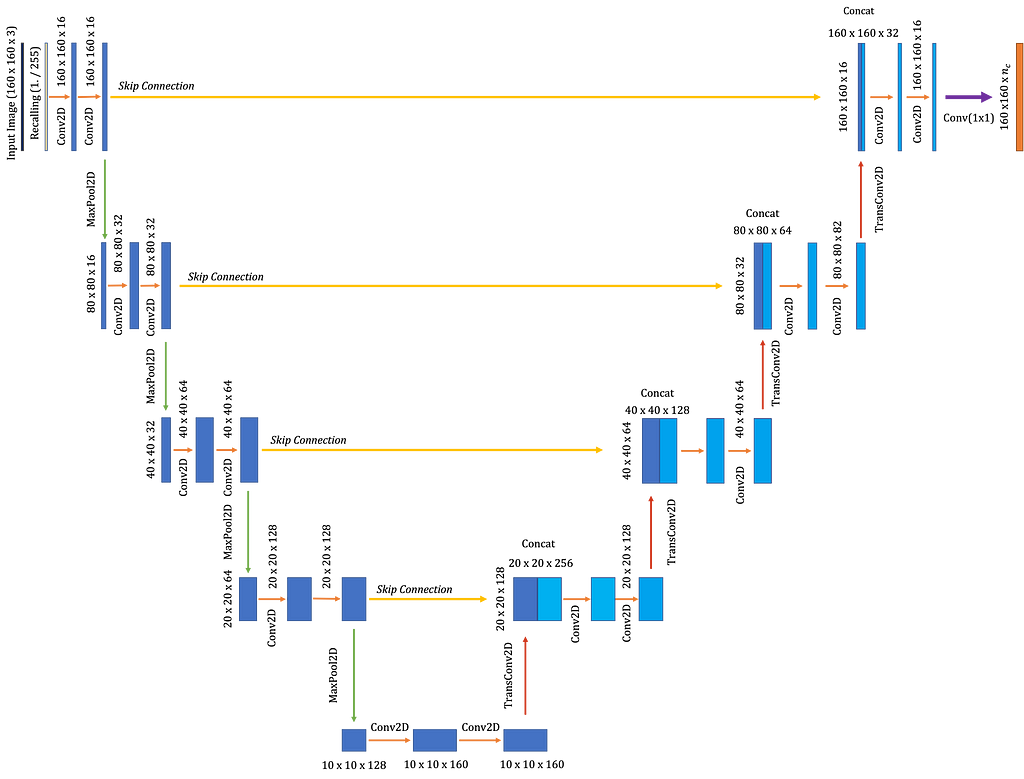
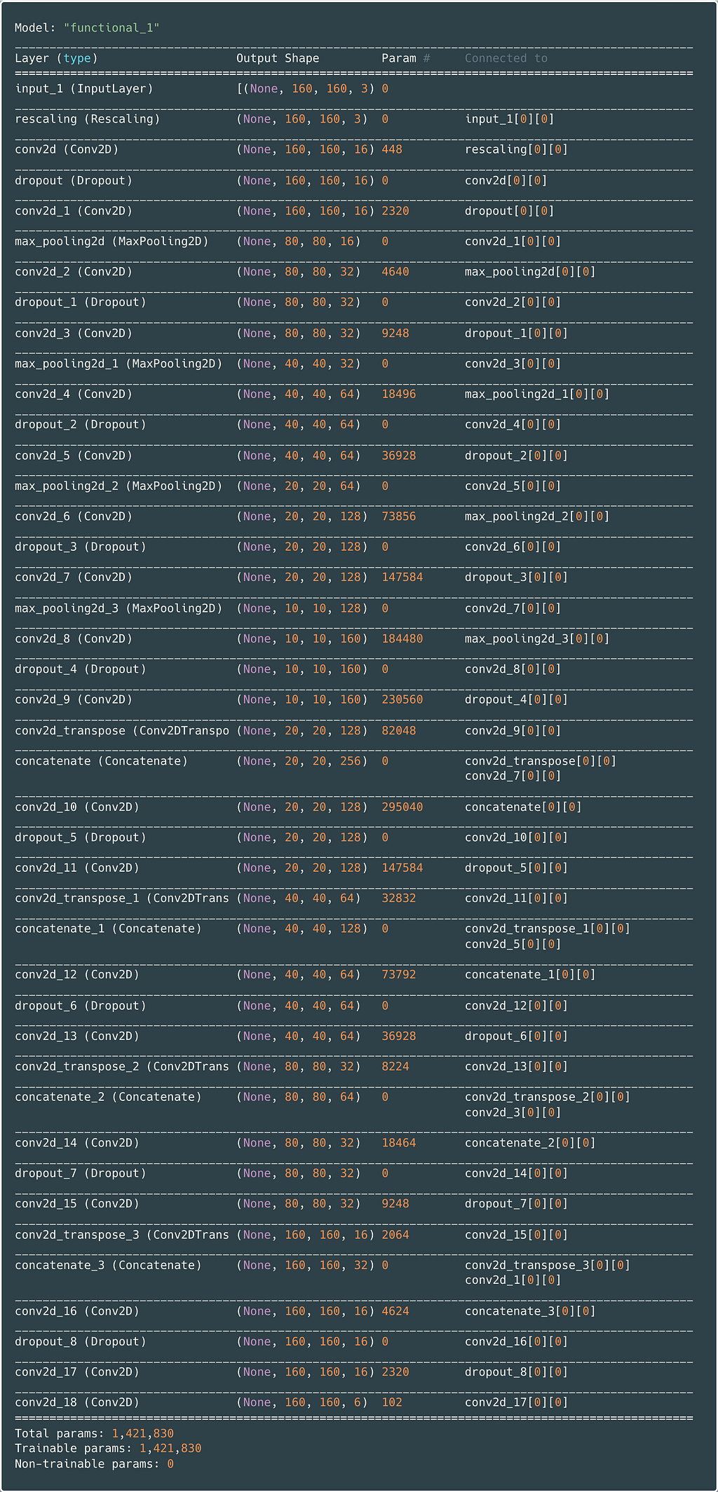
Figure 5 depicts the simple U-Net setup used for the aerial imagery segmentation and highlights all essential aspects of the network and layer shapes.
Two types of information allow U-Net to function optimally on semantic segmentation problems:
- Filters in the expansive path contain high level spatial and contextual feature information
- Detailed fine-grained structural information contained in the contraction path
Both of these elements fuse through the skip connection. Thus, the concatenation allows the neural network to use the high-resolution data accompanied by the low-level feature information to make predictions.
Gist 3 provides sample code to build a simple U-Net model using Keras.
Figure 6 provides the console log obtained using model.summary. Compare the Keras output with the architecture diagram in Figure 5 to see corresponding blocks and layer shapes.
Training and Evaluation
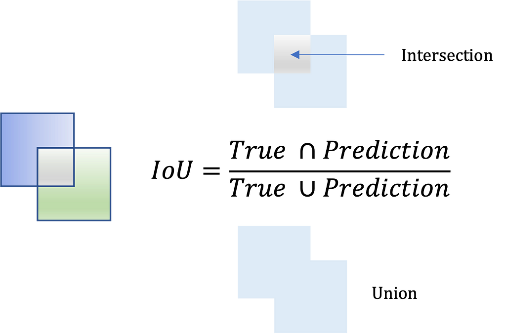
Performance metrics must be defined prior to fitting the training data. As image segmentation involves assigning a class to every pixel in a picture, a standard success indicator is the Intersection Over Union (IOU) coefficient.
IOU or Jaccard Index measures the number of overlapping pixels enclosed by the actual and predicted masks divided by the total pixels across both masks. Expression 3 calculates the IOU.
A custom Jaccard Similarity function is defined below in Gist 4.
Specific callbacks are helpful when training a neural network as they offer a view of the model’s internal state during training. Three callbacks defined in Gist 5 are:
- ModelCheckpoint: saves the best model out of all epochs with the highest validation_accuracy
- EarlyStopping: stops fitting if validation_loss does not continue to decrease over two epochs
- CSVLogger: saves model state values to a CSV file on each epoch
Once the callbacks are defined, the model compiles with Adam optimisation, categorical_crossentropy loss, and training initiates for 20 epochs with a batch_size=32 as seen in Gist 5.
Figure 7 is a copy of the Python console log returned during training. It shows the categorical_crossentropy loss decreasing on each iteration while the Jaccard similarity evaluation metric increases.
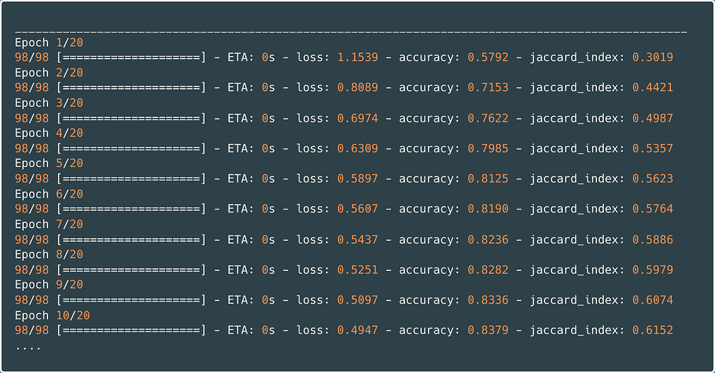
After training completion, the model is saved to the hard disk, having achieved the final performance index values:
- Loss ≈ 0.4170
- Accuracy ≈ 0.8616
- Jaccard Index ≈ 0.6599
Finally, use the code in Gist 6 to load the model with the necessary custom evaluation metrics defined as dependencies.
Prediction
Due to the dataset size limitations, predictions happen on randomly sampled images from the test set.
Detailed commented code to make predictions using the trained U-Net model is provided below in Gist 7.
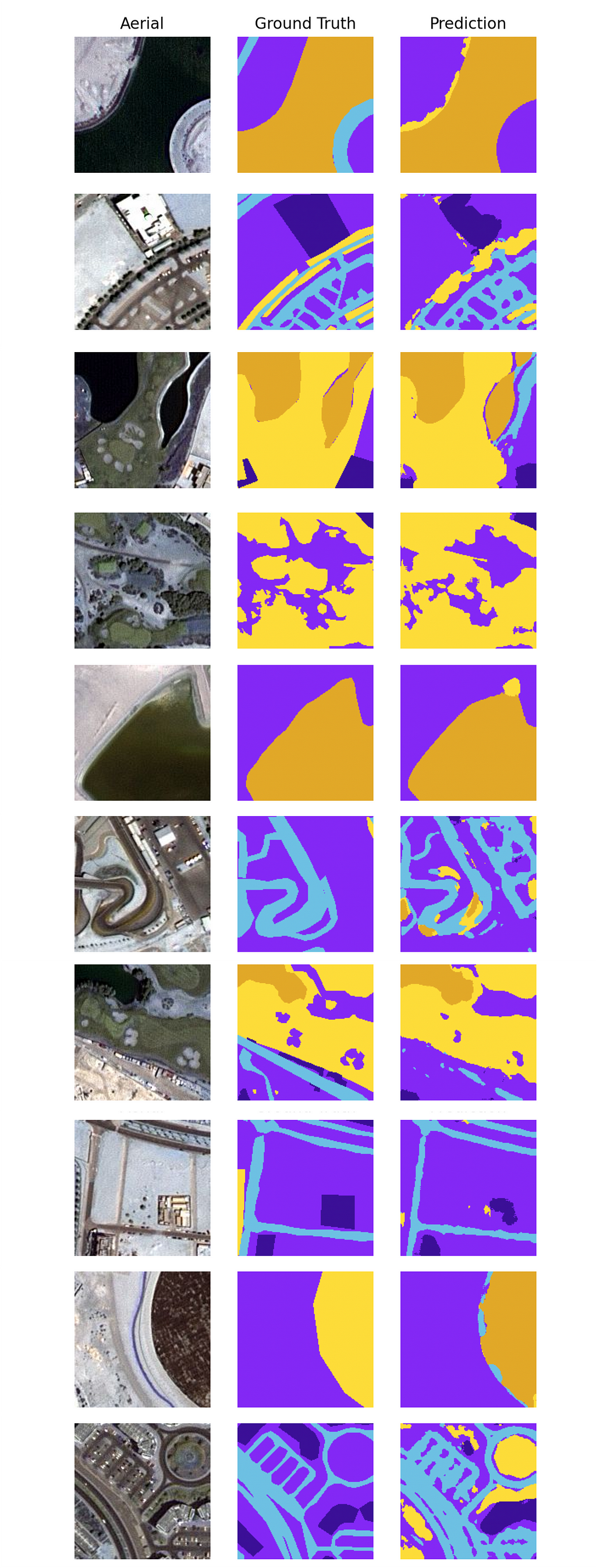
Figure 8 is a visualisation of ten outputs portraying the patched aerial image of Dubai, the ground truth mask and the U-Net segmentation prediction.
Conclusion
Due to limited computing power, the neural network size was restricted, and training iterations did not exceed 20 epochs. Currently, there are around 1.4 million trainable parameters, as shown in Figure 6. Therefore, model performance can undoubtedly be improved by hyperparameter tuning and employing a more sophisticated network.
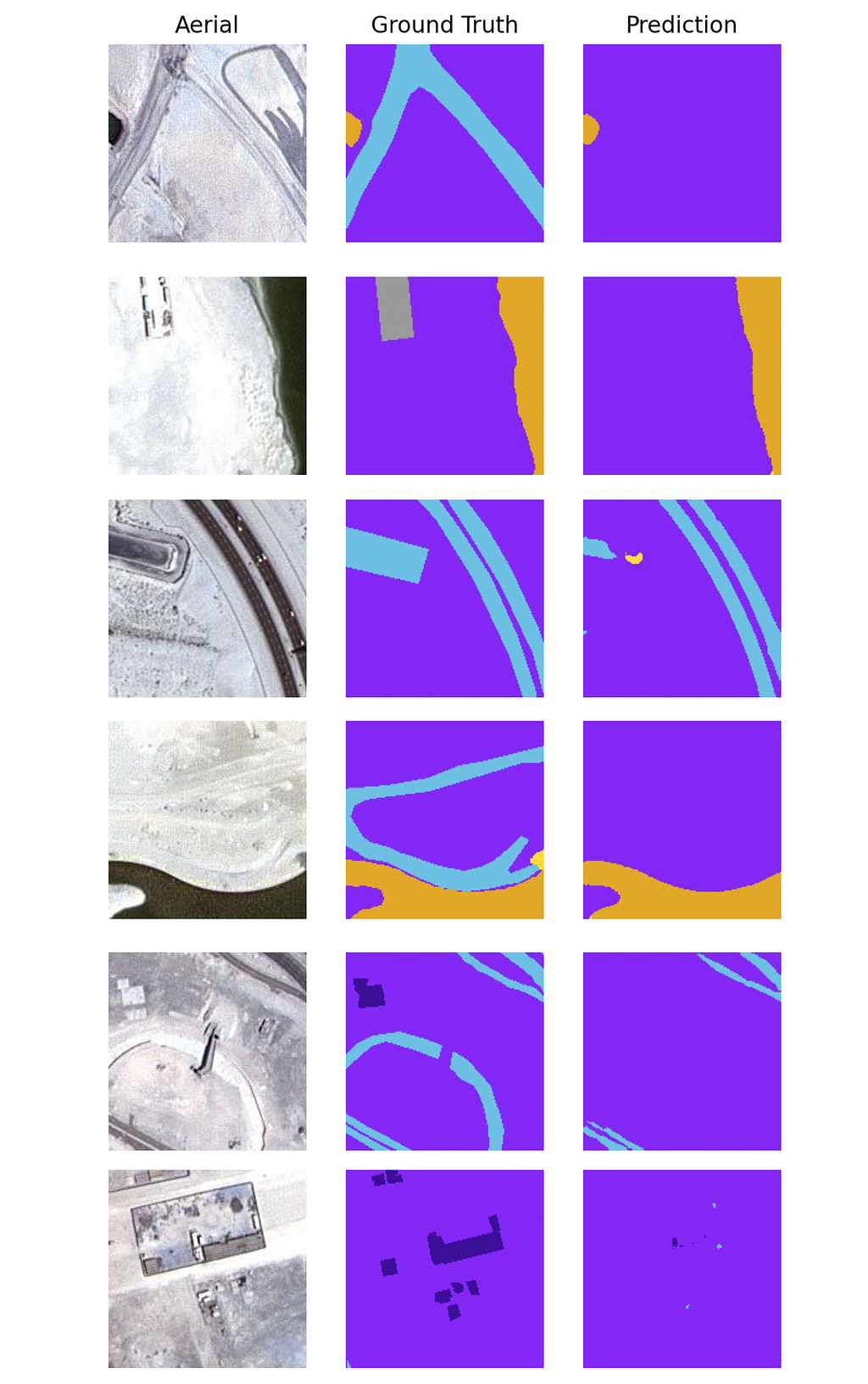
Figure 9 depicts some of the least successful segmentations. Some similarities are noticeable in the left-most column of aerial images. Each image is very bright, containing many pixels towards the white end of the RGB spectrum. Comparably, inspecting Figure 8, the most acceptable segmentations are on higher contrasted images. Therefore, it may be reasonable to synthesise additional brighter training images or fine-tune the model on a subset to improve performance.
Nevertheless, as the predictions show, the model generally performed relatively well given the small dataset size and limited computing capacity.
This article has demonstrated how to perform semantic segmentation on the MBRSC aerial imagery of the Dubai dataset using a U-Net TensorFlow model.
A similar process applies to other machine learning image segmentation tasks. U-Net was originally designed for work in the biomedical arena and, since its inception, has found use in various other fields.
References
[1] Semantic segmentation of aerial imagery (CC0: Public Domain) — Kaggle
[2] Convolutional Neural Networks — DeepLearning.AI, Andrew Ng
[3] Semantic segmentation of aerial (satellite) imagery using U-net — DigitalSreeni
[4] Evaluating Segmentation Models — Jeremy Jordan (May 30th 2018)
[5] Keras Callbacks Explained In Three Minutes — By Andre Duong, UT Dallas
Semantic Segmentation of Aerial Imagery using U-Net in Python was originally published in Towards Data Science on Medium, where people are continuing the conversation by highlighting and responding to this story.
from Towards Data Science - Medium https://ift.tt/jY0LgDT
via RiYo Analytics


ليست هناك تعليقات