https://ift.tt/30hye6l MACHINE LEARNING USING JULIA AND ITS ECOSYSTEM Part III — If things are not ‘ready to use’ Julia has a high degree...
MACHINE LEARNING USING JULIA AND ITS ECOSYSTEM
Part III — If things are not ‘ready to use’
Julia has a high degree of composability. With only a few lines of code new functionality can be built on top of existing packages.

Overview of the Tutorials
This is the third part of a tutorial that shows how Julia’s specific language features and a variety of high-quality packages from its ecosystem can be easily combined for use within a typical ML workflow.
- Part I “Analyzing the Glass dataset” concentrates on how data can be preprocessed, analyzed and visualized using packages like ScientificTypes, DataFrames, StatsBase and StatsPlots.
- Part II “Using a Decision Tree” focuses on the core of the ML workflow: How to choose a model and how to use it for training, predicting and evaluating. This part relies mainly on the package MLJ (= Machine Learning in Julia).
- Part III “If things are not ‘ready to use’” explains how easy it is to create your own solution with a few lines of code, if the packages available don’t offer all the functionality you need.
Introduction
In part two of the tutorial we created a decision tree and printed the following representation using print_tree():
Feature 3, Threshold 2.745
L-> Feature 2, Threshold 13.77
    L-> Feature 4, Threshold 1.38
        L-> 2 : 6/7
        R-> 5 : 9/12
    R-> Feature 8, Threshold 0.2
        L-> 6 : 8/10
        R-> 7 : 18/19
R-> Feature 4, Threshold 1.42
    L-> Feature 1, Threshold 1.51707
        L-> 3 : 5/11
        R-> 1 : 40/55
    R-> Feature 3, Threshold 3.42
        L-> 2 : 5/10
        R-> 2 : 23/26
It depicts the basic characteristics of the tree but is a bit rudimentary: It’s just ASCII-text and the nodes show only the attribute number, not the attribute name which is used for branching. Moreover, the leaves don’t show the class names, that get predicted at that point.
So it would be nice to have a graphical representation with all that additional information included. As there is no ready to use function for this purpose, we have to create one for ourselves. That’s what this third part of the tutorial is about.
The building blocks
What do we need to implement this by ourselves? Well, the following ingredients are surely the main building blocks:
- The decision tree itself (the data structure)
- Information about how this data structure looks like (internally)
- A graphics package with the ability to plot trees
… and of course, an idea, on how to glue these things together :-)
1. The decision tree
The MLJ function fitted_params() delivers for each trained machine all the parameters which result from training. Of course, this depends heavily on the model used. In case of a decision tree classifier one of these parameters is simply the tree itself:
fp = fitted_params(dc_mach)
typeof(fp.tree)     → DecisionTree.Node{Float64, UInt32}
2. Information about the data structure
In order to get some information about the internal structure of the decision tree, we have to look at the source code of the DecisionTree.jl package on GitHub.
There we find the following definitions for Leaf and Node:
This tells us, that the tree structure is made up of Nodes which store the number of the feature (featid) which is used for branching at that node and the threshold (featval) at which the branching took place. In addition each node has a left and a right subtree which is again a Node or a Leaf (if the bottom of the tree is reached).
The Leafs know the majority class (majority) which will be predicted when reaching this leaf as well as a list of all target values (values) that have been classified into this leaf.
3. A graphics package
The Julia graphics package Plots.jl by itself isn't capable of plotting trees. But there is a 'helper' package called GraphRecipes.jl which contains several so-called plotting recipes. These are specifications which describe how different graph structures can be plotted using Plots (or another graphics package that understands these recipes). Among other recipes, there is one for trees (called TreePlot).
The GraphRecipes serve also as an abstraction layer between a structure to be plotted and a graphics package that does the plotting.
Bringing it all together
The basic concepts
As we have the main building blocks identified now, the question remains of how we can fit these things together, to obtain the desired result. The main question is: How does the plot recipe TreePlot know, what our decision tree looks like in detail, so that it can be plotted by TreePlot? Both packages (DecisionTree.jl and GraphRecipes.jl) have been developed independently. They don't know anything about each other.
The documentation of TreePlot tells us, that it expects a structure of type AbstractTree (from the package AbstractTree.jl). But a decision tree from the DecisionTree.jl package doesn't conform to this type. So are we stuck now?
We would be stuck, if we were using an ‘ordinary’ object-oriented language. In this case we could perhaps try to define a new class which inherits from Node as well as from AbstractTree. But that works only, if the language supports multiple inheritance. If not, we could try to define a new class which inherits from AbstractTree and wrap somehow the Node and Leaf structures inside. All of this involves probably quite a bit of work and doesn't seem to be an elegant solution.
Fortunately we use Julia. Here we only have to (re-)define a few functions from AbstractTree on our decision tree, that makes it look like an AbstractTree. The TreePlot recipe expects only a specific behaviour from our decision tree (it really doesn't care about the type of this data structure): It wants the tree to have
- a function children(t) that, when applied to the tree t (or to a node of the tree), returns a list of its subtrees
- and a function printnode(io::IO, node) that prints a representation of the node node to the output stream io.
The following diagram shows all these components and how they are related:
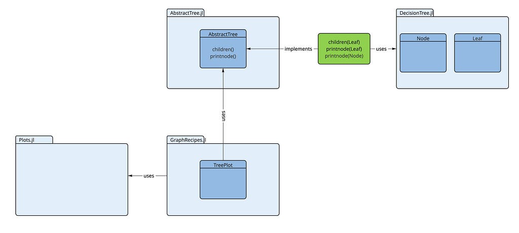
We only have to create the part depicted in green (the blue ones already exist). That’s all we need. Then the decision tree conforms to an AbstractTree (as far as TreePlot is concerned). So let's do it:
A first and simple implementation
This can be done with the following few lines of code:
As we use some type and function definitions from the packages DecisionTree and AbstractTree, we have to declare their usage (with import or using).
The implementation of children is a simple one-line function which just returns the left and the right subtree.
For printing we have to differentiate between nodes and leafs, because the output of a node looks different from that of a leaf. In most programming languages we would need an implementation that checks the type of the node/leaf to be printed and use an if ... then ... else-statement in this case. Not so in Julia! Here we can use its multiple dispatch capability and implement two versions of printnode: One for Nodes and another one for Leafs. Julia chooses automatically the correct one, depending on the type of the second parameter.
Here we have chosen a very simple implementation for printnode as a first step. The version for Node prints the same information as does the built-in print_tree() which we've used above (the ID of the feature and the threshold). The variant for Leaf is even simpler: It prints the ID of the predicted class and the number of values under consideration in this leaf.
The AbstractTree.jl package also has a function print_tree which does a text-based output of a tree using the two functions we've implemented above. Let's use AbstractTree.print_tree to test our first implementation:
AbstractTrees.print_tree(fp.tree) -->
Feature: 3 — Threshold: 2.745
├─ Feature: 2 — Threshold: 13.77
│ ├─ Feature: 4 — Threshold: 1.38
│ │ ├─ maj: 2 — vals: 7
│ │ └─ maj: 5 — vals: 12
│ └─ Feature: 8 — Threshold: 0.2
│   ├─ maj: 6 — vals: 10
│   └─ maj: 7 — vals: 19
└─ Feature: 4 — Threshold: 1.42
  ├─ Feature: 1 — Threshold: 1.51707
  │ ├─ maj: 3 — vals: 11
  │ └─ maj: 1 — vals: 55
  └─ Feature: 3 — Threshold: 3.42
    ├─ maj: 2 — vals: 10
    └─ maj: 2 — vals: 26
Looks pretty good and all values correspond to the ones in our first printout of the decision tree above. So the implementation seems to work flawlessly!
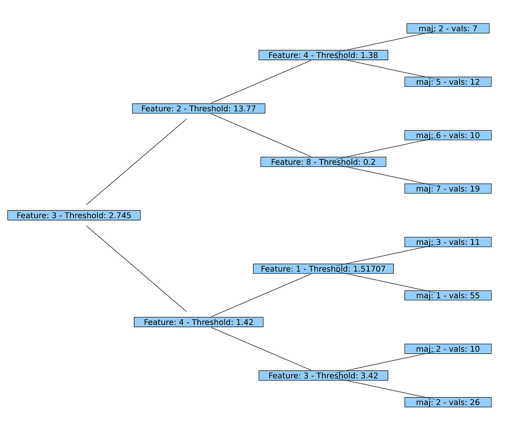
And now the graphical representation using Plots and GraphRecipes: As we already have implemented the necessary functions, we can just call plot using a TreePlot (applying the Buchheim tree layout algorithm). That's it!
using GraphRecipes
plot(TreePlot(fp.tree),
        method = :buchheim, nodeshape = :rect,
        root = :left, curves = false)
Fine tuning the output
In the next step we want a tree which shows feature names on its nodes and the names of the predicted classes on its leafs (instead of the IDs used before). Unfortunately a DecisionTree doesn't know this information at all. I.e. we have to add that information somehow so that they can be used by the mechanisms applied in the last section.
The idea is to add this information while traversing the decision tree using children, so that printnode has access to it. That's the only place where we need this information. There is no need to change the decision tree structures in any way.
So, instead of returning the Node and Leaf structures from DecisionTree directly, children will return enriched structures with added information. These enriched structures are defined as follows:
The attribute info within these new structs may contain any information we like to show on the printed tree. dt_node and dt_leaf are simply the decision tree elements we already used before.
In order to create these enriched structures on each call of children, we define a function wrap_element() with two implementations: One to create a NamedNode and a second one to create a NamedLeaf. This is another situation where we rely on the multiple dispatch mechanism of Julia. Depending on the type of the second argument (a Node or a Leaf) the correct method will be chosen.
This makes the implementation of our new children function quite easy: Just two calls to wrap_element(), where we add the attribute names and the class names as parameters (as a NamedTuple; a Julia standard type which comes in handy here).
The implementations of printnode receive now a NamedNode or a NamedLeaf and can use the information within these elements for printing:
The variable matches (in the second implementation of printnode) contains the instances which have been correctly classified on this leaf (out of all instances on this leaf in values). So the ratio of correctly classified instances vs. all instances (match_count vs. val_count) can be shown.
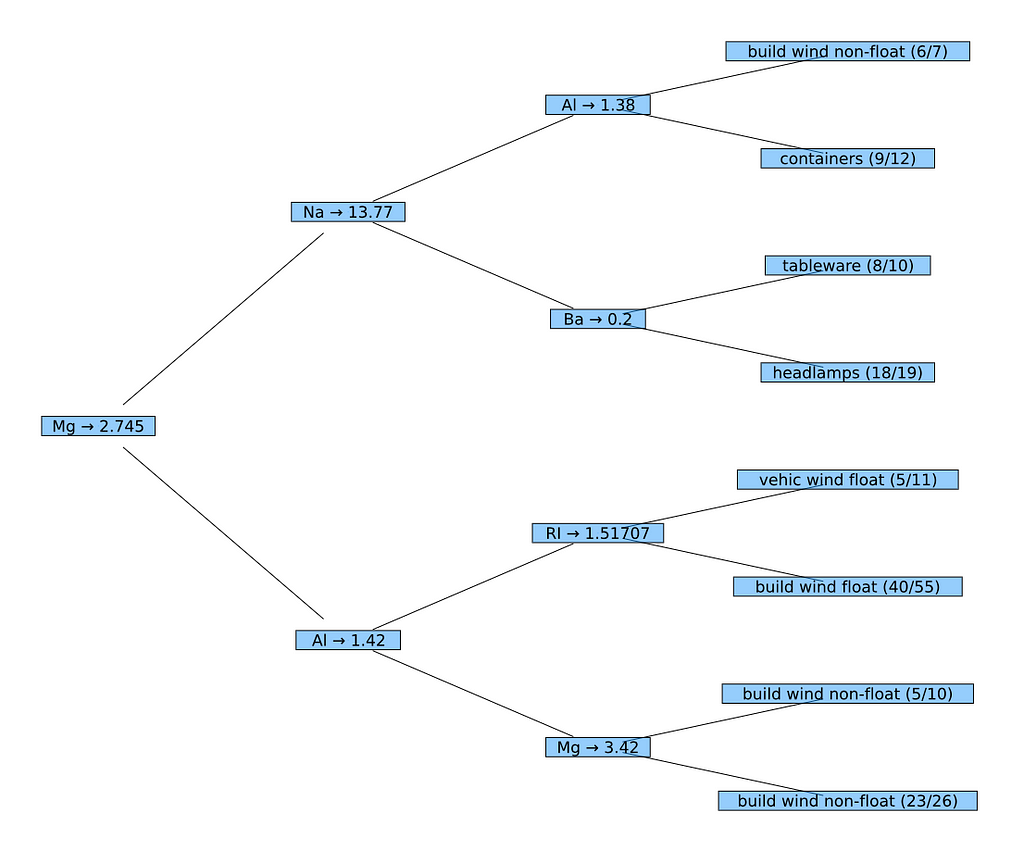
To plot the decision tree, we finally create a NamedNode for the root of the decision tree. Then we use again plot with the TreePlot recipe to obtain the desired result.
nn = NamedNode(
        (atr = names(XGlass), cls = levels(yGlass)),
        fp.tree)
plot(TreePlot(nn),
        method = :buchheim, nodeshape = :rect,
        root = :left, curves = false)
Conclusions
The examples above demonstrated that it is possible to combine several unrelated Julia packages with just a few lines of code, thus creating new, useful functionality.
Especially the second example (“fine tuning …”) has of course some potential for optimization with respect to (memory) efficiency and modularity/reuse. But this can also be done with only a little more effort.
Further information
On GitHub (in: roland-KA/JuliaForMLTutorial) I’ve made available Pluto notebooks for all three parts of this tutorial with full code examples. So everybody is invited to try it out for themselves.
Part III — If things are not ‘ready to use’ was originally published in Towards Data Science on Medium, where people are continuing the conversation by highlighting and responding to this story.
from Towards Data Science - Medium https://ift.tt/6Sxkv7j
via RiYo Analytics


ليست هناك تعليقات