https://ift.tt/rG4ngts How to automate data preparation and save time on your next data science project Image from Unsplash . It is com...
How to automate data preparation and save time on your next data science project

It is commonly known among Data Scientists that data cleaning and preprocessing make up a major part of a data science project. And, you will probably agree with me that it is not the most exciting part of the project.
So, (let’s ask ourselves): can we automate this process?
Well, automating data cleaning is easier said than done, since the required steps are highly dependent on the shape of the data and the domain-specific use case. Nevertheless, there are ways to automate at least a considerable part of it in a standardized way.
In this article, I will show you how you can build your own automated data cleaning pipeline in Python 3.8.
View the AutoClean project on Github.
1 | What do we want to Automate?
The first and most important question we should ask ourselves before diving into this project is: which steps of the data cleaning process can we actually standardize and automate?
Steps that can most likely be automated or standardized, are steps which are performed over and over again, in each cleaning process of almost every data science project. And, since we want to build a “one size fits all” pipeline, we want to make sure that our processing steps are fairly generic and can adapt to various types of datasets.
For example, some of the common questions that are repeatedly asked during the majority of projects include for example:
- What format does my data come in? CSV, JSON, text? Or another format? How am I going to handle this format?
- What data types do our data features come in? Does our dataset contain categorical and/or numerical data? How do we deal with each? Do we want to one-hot encode our data, and/or perform data type transformations?
- Does our data contain missing values? If yes, how do we deal with them? Do we want to perform some imputation technique? Or can we safely delete the observations with missing values?
- Does our data contain outliers? If yes, do we apply a regularization technique, or do we leave them as they are? …and wait, what do we even consider as an “outlier”?
No matter what use case our project will be targeted at, these are questions that will very likely need to be addressed, and therefore can be a great subject of automation.
The answers to these questions, as well as their implementation will be discussed and shown in the next few chapters.
2 | Building Blocks of the Pipeline
First off, let’s start by importing the libraries we will be using. Those will be mainly the Python Pandas, Sklearn and Numpy library, as these are very helpful when it comes to manipulating data.
We will define that our script will take a Pandas dataframe as input, which means that we need to at least transform the data into a Pandas dataframe format before it can be processed by our pipeline.
Now let’s look at the building blocks of our pipeline. The below chapters will go through the following processing steps:
[Block 1] Missing Values
[Block 2] Outliers
[Block 3] Categorical Encoding
[Block 4] Extraction of DateTime Features
[Block 5] Polishing Steps
[ Block 1 ] Missing Values
It is fairly common that a project starts with a dataset that contains missing values and there are various methods of dealing with them. We could simply delete the observations containing missing values, or we can use an imputation technique. It is also common practice to predict missing values in our data with the help of various regression or classification models.
💡 Imputation techniques replace missing data by certain values, like the mean, or by a value similar to other sample values in the feature space (f. e. K-NN).
The choice of how we handle missing values will depend mostly on:
- the data type (numerical or categorical) and
- how many missing values we have relative to the number of total samples we have (deleting 1 observation out of 100k will have a different impact than deleting 1 out of 100)
Our pipeline will follow the strategy imputation > deletion, and will support the following techniques: prediction with Linear and Logistic Regression, imputation with K-NN, mean, median and mode, as well as deletion.
Good, now we can start writing the function for our first building block. We will first create a separate class for handling missing values. The function handle below will handle numerical and categorical missing values in a different manner: some imputation techniques might be applicable only for numerical data, whereas some only for categorical data. Let’s look at the first part of it which handles numerical features:
This function checks which handling method has been chosen for numerical and categorical features. The default setting is set to ‘auto’ which means that:
- numerical missing values will first be imputed through prediction with Linear Regression, and the remaining values will be imputed with K-NN
- categorical missing values will first be imputed through prediction with Logistic Regression, and the remaining values will be imputed with K-NN
For categorical features, the same principle as above applies, except that we will support only imputation with Logistic Regression, K-NN and mode imputation. When using K-NN, we will first label encode our categorical features to integers, use these labels to predict our missing values, and finally map the labels back to their original values.
Depending on the handling method chosen, the handle function calls the required functions from within its class to then manipulate the data with the help of various Sklearn packages: the _impute function will be in charge of K-NN, mean, median and mode imputation, _lin_regression_impute and log_regression_impute will perform imputation through prediction, and I assume that the role of _delete is self-explanatory.
Our final MissingValues class structure will look as following:
I will not go more into detail on the code within the remaining functions of the class, but I invite you to check out the full source code in the AutoClean repository.
After we have finished all the required steps, our function then outputs the processed input data.
Cool, we made it through the first block of our pipeline 🎉. Now let’s think about how we will handle outliers in our data.
[ Block 2 ] Outliers
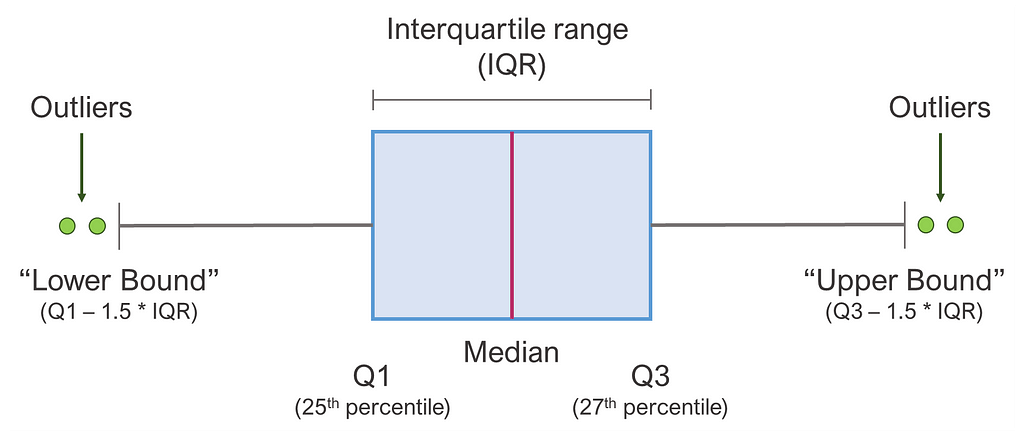
Our second block will focus on the handling of outliers in our data. First we need to ask ourselves: when do we consider a value to be an outlier? For our pipeline, we will use a commonly applied rule that says that a data point can be considered an outlier if is outside the following range:
[Q1 — 1.5 * IQR ; Q3 + 1.5 * IQR]
…where Q1 and Q3 are the 1st and the 3rd quartiles and IQR is the interquartile range. Below you can see this nicely visualized with a boxplot:
Now that we have defined what an outlier is, we now have to decide how we handle these. There are again various strategies to do so, and for our use-case we will focus on the following two: winsorization and deletion.
💡 Winsorization is used in statistics to limit extreme values in the data and reduce the effect of outliers by replacing them with a specific percentile of the data.
When using winsorization, we will again use our above defined range to replace outliers:
- values > upper bound will be replaced by the upper range value and
- values < lower bound will be replaced by the lower range value.
The final structure of our Outliers class will look as following:
We arrived at the end of the second block — now let’s have a look at how we can encode categorical data.
[ Block 3 ] Categorical Encoding
In order to be able to perform computations with categorical data, in most cases we need our data to be of a numeric type i. e. numbers, or integers. Therefore, common techniques consist of one-hot encoding data, or label encoding data.
💡 One-hot encoding of data represents each unique value of a feature as a binary vector, whereas label encoding assigns a unique integer to each value.
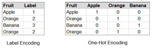
There are various pros and cons for each of the methods, like f. e. the fact that one-hot encoding produces a lot of additional features. Also, if we label encode, the labels might be interpreted by certain algorithms as mathematically dependent: 1 apple + 1 orange = 1 banana, which is obviously a wrong interpretation of this type of categorical data.
For our pipeline, we will set the default strategy ‘auto’ to perform the encoding according to the following rules:
- if the feature contains < 10 unique values, it will be one-hot-encoded
- if the feature contains < 20 unique values, it will be label-encoded
- if the feature contains > 20 unique values, it will not be encoded
This is quite a primitive and quick way of handling the encoding process which might come in handy, but might also lead to encodings not fully appropriate for our data. Even though automation is great, we still want to make sure that we can also define manually which features should be encoded, and how. This is implemented in the handle function of the EncodeCateg class:
The handle function takes a list as input, whereas the features we want to manually encode can be defined by column names or indexes as following:
encode_categ = [‘onehot’, [‘column_name’, 2]]
Now that we’ve defined how to handle outliers, we can move on to our fourth block, which will cover the extraction of datetime features.
[ Block 4 ] Extraction of DateTime features
If our dataset contains a feature that has datetime values, like timestamps or dates, we will very likely want to extract these so they become easier to handle when processing or visualizing later on.
We can also do this in an automated fashion: we will let our pipeline search through the features and check whether one of these can be converted into the datetime type. If yes, then we can safely assume that this feature holds datetime values.
We can define the granularity at which the datetime features are extracted, whereas the default is set to ‘s’ for seconds. After the extraction, the function checks whether the entries for dates and times are valid meaning: if the extracted columns ‘Day’, ‘Month’ and ‘Year’ all contain 0’s, all three will be deleted. The same happens for ‘Hour’, ‘Minute’ and ‘Sec’.
Now that we are done with datetime extraction we can move on to the last building block of our pipeline which will consist of some final adjustment to polish our output dataframe.
[ Block 5 ] Dataframe Polishing
Now that we’ve processed our dataset, we still need to do a few adjustments to make our dataframe ‘look good’. What do I mean by that?
Firstly, some features that were originally of type integer could have been converted to floats, due to imputation techniques or other processing steps that were applied. Before outputting our final dataframe we will convert these values back to integers.
Secondly, we want to round all the float features in our dataset to the same number of decimals as they had in our original input dataset. This is to avoid on one hand unnecessary trailing 0’s in the float decimals, and on the other hand make sure not to round our values more than our original values.
Again, I will not go more into detail on the code behind these ideas, but I invite you to check out the full source code in the AutoClean repository.
3 | Putting it all Together
First of all, congrats for sticking with me this far! 🎉
We’ve now arrived at the part where we want to put all of our building blocks together so we can actually start using our pipeline. Instead of posting the full code here, you will find the full AutoClean code in my GitHub repository:
GitHub - elisemercury/AutoClean: Package for automated data cleaning in Python.
Let’s look at a visual example of how AutoClean processes the sample dataset below:
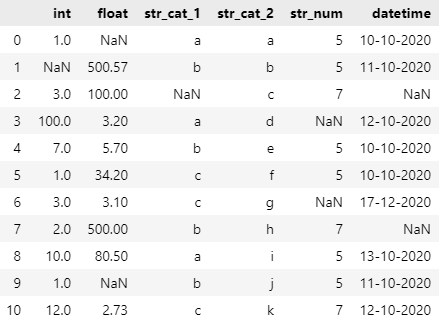
I generated a random dataset, and as you can see, I made it fairly varying when it comes to the different data types and I added a few random NaN values in the dataset.
Now we can run the AutoClean script as following:
The resulting cleaned output dataframe looks as below:
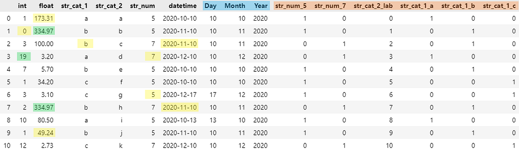
In the image above you will see visualized which changes AutoClean made to our data. The imputed missing values are marked in yellow, the outliers in green, the extracted datetime values in blue and the categorical encodings in orange.
I hope this article was informative for you and that AutoClean will help you save some valuable minutes of your time. 🚀
Feel free to leave comment if you have any questions or feedback. Contributions on GitHub are also welcome!
References:
[1] N. Tamboli, All You Need To Know About Different Types Of Missing Data Values And How To Handle It (2021)
[2] C. Tylor, What Is the Interquartile Range Rule? (2018)
[3] J. Brownlee, Ordinal and One-Hot Encodings for Categorical Data (2020)
Automated Data Cleaning with Python was originally published in Towards Data Science on Medium, where people are continuing the conversation by highlighting and responding to this story.
from Towards Data Science - Medium https://ift.tt/150PzD8
via RiYo Analytics


ليست هناك تعليقات