https://ift.tt/qbfX2Mn And a Python tutorial to get you up and running with the RE model on a real world data set The Random Effects regre...
And a Python tutorial to get you up and running with the RE model on a real world data set
The Random Effects regression model is used to estimate the effect of individual-specific characteristics such as grit or acumen that are inherently unmeasurable. Such individual-specific effects are often encountered in panel data studies. Along with the Fixed Effect regression model, the Random Effects model is a commonly used technique to study the effect of individual-specific features on the response variable of the panel data set.
For those of you who have read my articles on the Fixed Effects model and the Pooled OLS model, the first 10% of this article might feel like a revision of concepts.
Let’s begin by briefly (re)acquainting ourselves with panel data sets.
What is a panel data set?
A panel data set contains data about a set of uniquely identifiable individuals or “things” that are actively tracked over a period of time. Each individual or “thing” is called a unit. Examples of what can be considered a tracked unit are a person, family, tree, vehicle, company and country. Typically, for each unit, one measures one or parameters (a.k.a. regression variables or effects) in each time period.The set of data points pertaining to one unit (one country) is called a group.
If all units are tracked for the same number of time periods, the data panel is called a balanced panel. Otherwise, it’s called an unbalanced panel. If the same set of units is tracked throughout the study, it’s called a fixed panel, but if the units change during the study, it’s called a rotating panel.
Panel data sets usually arise out of what are known longitudinal studies such as the Framingham Heart Study or the The British Household Panel Survey.
The World Bank panel data set
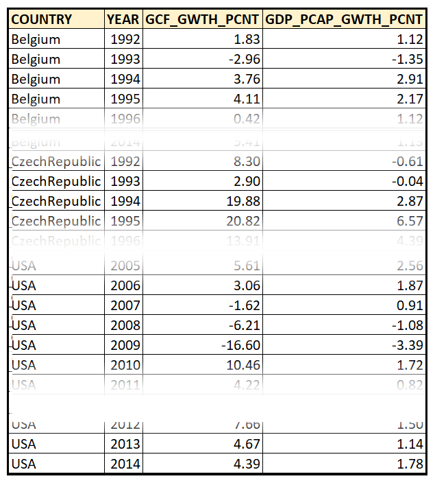
In this article, we’ll use a panel data set drawn from the World Bank containing data on Year-over-Year % growth in per capita GDP, and Y-o-Y % growth in Gross Capital Formation for seven countries. This data was captured from 1992 through 2014. Here is how this panel data set looks like:
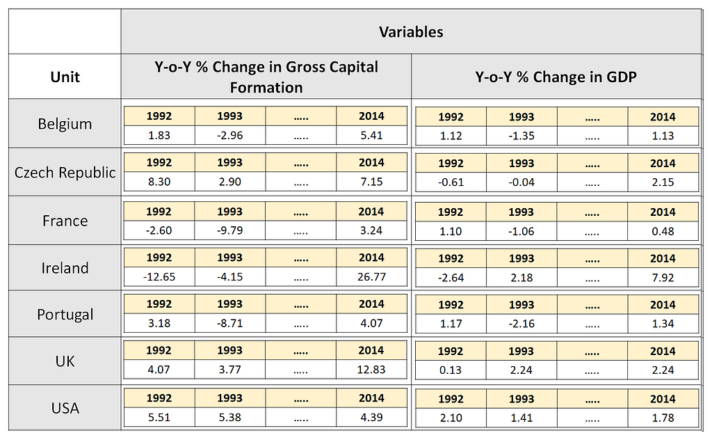
In the above data set, the unit is a country, and there are two variables: GDP growth and GCF growth. So, we are tracking 2 variables for each of the 7 units over 23 time periods (1992 through 2014). This results in the creation of 7 groups of data. The World Bank data set is fixed and balanced.
Regression goal
Our goal will be to study the influence of Y-o-Y % growth in gross capital formation on Y-o-Y % growth in GDP.
Therefore, our dependent or response variable y is Y-o-Y % growth in per capita GDP.
The independent or explanatory variable X is Y-o-Y % growth in gross capital formation.
We’ll begin by visually inspecting the relationship between GDP growth and GCF growth.
Let’s create a scatter plot of y versus X to see how the data looks like.
We’ll start by importing all the required Python packages including ones we would use later on to construct the Random Effects model.
import pandas as pd
import scipy.stats as st
import statsmodels.api as sm
import statsmodels.formula.api as smf
from matplotlib import pyplot as plt
import seaborn as sns
Let’s load the data set into a Pandas Data frame. The data set is available for download over here.
df_panel = pd.read_csv('wb_data_panel_2ind_7units_1992_2014.csv', header=0)
We’ll use Seaborn to plot per capita GDP growth across all time periods and across all 7 countries versus gross capital formation growth in each country:
colors = ['blue', 'red', 'orange', 'lime', 'yellow', 'cyan', 'violet']
sns.scatterplot(x=df_panel['GCF_GWTH_PCNT'],
                y=df_panel['GDP_PCAP_GWTH_PCNT'],
                hue=df_panel['COUNTRY'],
                palette=colors).
                set(title='Y-o-Y % Change in per-capita GDP versus Y-o-Y % Change in Gross capital formation')
plt.show()
We see the following plot:
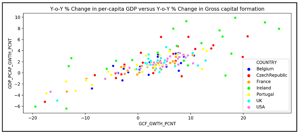
The relation between GDP and GCF growth appears to be linear, although there is also quite a lot of heteroskedasticity in the data.
As a working hypothesis, let’s assume the following linear functional form for the relationship between:
y=Y-o-Y % growth in per capita GDP, and,
X=Y-o-Y % growth in gross capital formation

The above equation is a matrix equation as indicated by the bold font style for the variables. Assuming there are T time periods per group, k regression variables per unit and n units, the dimensions of each matrix variable in the equation are as follows:
- y_i is the response variable for unit i. It is a vector of size [T x 1].
- X_i is the regression variables matrix of size [T x k].
- β_i is the coefficients matrix of size [k x 1] containing the population (true) value of the coefficients for the k regression variables in X_i.
- ϵ_i is a matrix of size [T x 1] containing the error terms of the model, one error term for each of the T time periods. An error term is defined as the difference between the observed value and the ‘modeled’ value.
Following is the matrix form of this equation:

In the World Bank panel data set, T=23, k=1 and n=7.
In the above regression model, the error terms ϵ_i arise out of a number of reasons such as follows:
- Measurement errors,
- Random noise in the experimental setup,
- Errors introduced due to the accidental or deliberate omission of one or relevant explanatory variables,
- Incorrect choice of regression model or incorrect choice of functional form for the regression variables or the response variable in the model,
- Errors introduced due to our inability to measure certain characteristics that are unit-specific. In the countries data panel, such unit-specific effects could be the socioeconomic fabric of the country that fuels or inhibits GDP growth under different environmental circumstances, and cultural aspects of decision-making in business and government that have evolved over hundreds of years in that country.
The unit-specific effects are inherently unmeasurable (some authors prefer to call them unobservable effects).
We still need to find a way to measure their effects on the response variable because if we entirely omit them from the regression analysis, their effect will leak into the error terms (and therefore into the residual errors of the trained model) in an uncontrolled way and make our model sub-optimal.
To that end, we will begin by restating the regression model’s equation for unit (i.e. country) i as follows:

In the above equation:
- y_i is a matrix of size [T x 1] containing the T observations for country i.
- X_i is a matrix of size [T x k] containing the values of k regression variables all of which are observable and relevant.
- β_i is a matrix of size [k x 1] containing the population (true)values of regression coefficients for the k regression variables.
- Z_i is a matrix of size [T x m] containing the (theoretical) values of all the variables (m in number) and effects that cannot be directly observed.
- γ_i is a matrix of size [m x 1] containing the (theoretical) population values of regression coefficients for the m unobservable variables.
- ε_i is a matrix of size [T x 1] containing the error terms corresponding to the T observations for country i.
Here is how the matrix multiplications and additions look like:

All unit-specific effects are assumed to be introduced by the term Z_iγ_i. The matrix Z_i and its coefficients vector γ_i are purely theoretical terms since what they represent cannot be in reality observed and measured.
Our objective is to find a way to estimate the impact of all unobservable effects contained in Z_i on y, i.e. the impact of Z_iγ_i on y_i.
To simplify the estimation, we’ll combine the effect of all country-specific unobservable effects into one variable which we will call z_i for country i. z_i is a matrix of size [T x 1] since it contains only one variable z_i and it has T rows corresponding to T number of “measurements”, each one of value z_i.
Since z_i are not directly observable, in order to measure the effects of z_i, we need to formalize the effect of leaving out z_i. To do so, we will appeal to a concept in statistics called the omitted-variable bias.
Omitted variable bias
While training the model on the panel data set, if we leave out z_i from the model, it will cause what is known as the omitted variable bias. It can be shown that if the regression model is estimated without considering z_i, then the estimated values β_cap_i of the model coefficients β_i will be biased in the following manner:
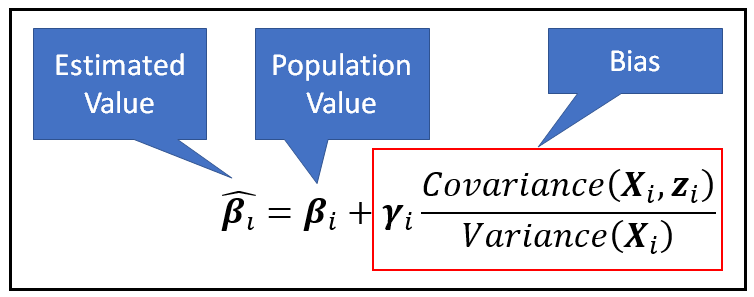
In the above equation, it can be seen that the bias introduced in the estimated value β_cap_i is directly proportional to the covariance between the omitted variable z_i and the explanatory variables X_i. This suggests a motivation for two building kinds of regression models:
- A Fixed Effects model in which the covariance is non-zero, i.e. the unit-specific effects are correlated with the regression variables, and,
- A Random Effects model in which the covariance term is zero, i.e. the unit-specific effects are independent of the regression variables.
In a previous article, we saw how to construct the Fixed Effects model. In this article, we’ll focus on the Random Effects model and compare its performance with both the FE model and the Pooled OLS Regression model.
The Random Effects model
To understand the structure of the Random Effects model, it can be useful to start with the structure of the FE model, and contrast it with that of the RE model. So, let’s briefly recap the structure of the Fixed Effects model.
The key assumption of the Fixed Effects model is that the unobservable effects are correlated with the regression variables of the model. In the section on the omitted variable bias we saw that the presence of such a correlation will cause the covariance term to be non-zero, which will in turn cause the bias to be proportional to absolute value of this covariance. To counter this bias, the Fixed Effects model takes the approach of introducing a unit-specific bias term c_i into the regression equation as follows:

Notice that we have replaced the term z_iγ_i that contributes all the known unit-specific effects with c_i which is a matrix of size [T x 1] in which each element has the same value c_i. Also, c_i is constant across all time periods in the data panel.
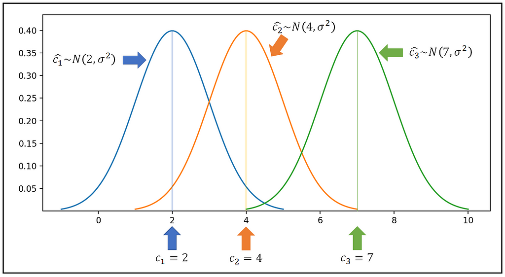
The estimated value of c_i, namely (we’ll call it c_cap_i) is a random variable that has a certain probability distribution having a mean of c_i. In the Fixed Effects model, we assume that the estimated value of all unit specific effects have the same constant variance σ². It is also convenient (although not necessary) to assume a normally distributed c_cap_i. Thus, we have:
c_cap_i ~ N(c_i, σ²)
The following figure illustrates the distributions for c_i for three units:
Now let us come to the motivation for the Random Effects model.
If the unit-specific effect is not correlated with the regression variables, then the effect becomes entirely part of the error term ϵ. We can no longer use the strategy that we used in the Fixed Effects model to compensate for its absence, i.e. we can no longer assume the existence of a distinct, unit-specific effect c_i whose effect will compensate for the bias that would have been introduced by the omission of all the unobserved variables z_i from the model.
Therefore, we need a different way to account for unit-specific effects, and for that, we take recourse to an ingenious modeling approach.
Recollect the following regression equation:

Recollect that the term Z_iγ_i produces the unit-specific effect. Z_iγ_i happens to be a random variable having some mean and variance.
In the Random Effects model, we assume that the unit-specific effects for all units are distributed around a common mean value according to some unknown probability distribution. Furthermore, this common mean is constant across all time periods in the data panel.
Notation-wise, these assumptions give rise to the following conditional expectation for the term Z_iγ_i that’s meant to capture all unobservable unit-specific effects:
E( Z_iγ_i | X_i) = α
Now, let’s add and subtract this expected value from the R.H.S. of the model’s regression equation:

In the above equation, the term ( Z_iγ_i — E( Z_iγ_i | X_i)) is the variation of the unit-specific effect around its mean. We will designate this variation by the term μ_i.
Furthermore, we have already assumed that the yellow term in the above equation which is the expected value of all unit-specific effects have a constant value of α, i.e. E( Z_iγ_i | X_i) = α.
Thus, we arrive at the following equation for the Random Effects regression model:

The above equation suggests the following insight:
While estimating the model’s parameters, if we were to leave out the unit-specific effects Z_iγ_i, we would be introducing two things:
- A constant α that captures the mean of all unit-specific effects. This mean does not vary with time and it effectively takes the place of the regression model’s intercept term.
- An error term μ_i whose magnitude is proportional to the variance of the unit-specific effect around the constant mean.
Taking this perspective gives us the reason for combining u_i with the error term ϵ_i to form a composite error term that we have shown in the bracket.
This composite error term is a defining characteristic of a Random Effects regression model. As we shall soon see, the individual components of the composite error term need to be estimated as part of the estimation procedure of the RE model.
Following is the Random Effect model’s equation for unit i and for a specific time period t:

In the above equation:
- y_i_t is the value of the response variable (% GDP growth in the WB data set) of unit (country) i at time period (year) t.
- x_i_t is a row vector of size [1 x k] assuming k regression variables (k=1 for the WB data panel). x_i_t is the t-th row in the X_i regression matrix which we looked at earlier which is of size [T x k].
- β_i is a column vector of size [k x 1]. In the WB data set, there is only one regression variable: % gross capital formation growth.
- α is the common bias (the mean of all unit-specific effects). It forms the intercept of the linear regression model.
- μ_i is the variance introduced by the unit-specific effect for unit i. Notice that it lacks the time subscript t as it is assumed to be constant across all time periods in the data panel (a.k.a. time invariant).
- ϵ_i_t is the balance amount of error from all other sources introduced for unit i at time period t.
Here is the matrix form of the above equation:

Characteristics of the composite error term of the Random Effects model
The RE model’s composite error term has a few important characteristics that determine how these errors are estimated.
- As with the Fixed Effects model, the error ϵ_i_t is a random variable that is assumed to fluctuate around a mean value of zero with some unknown (but often assumed to be normal) probability distribution. Thus, the conditional expectation of the errors is zero:
E(ϵ_i_t|X_i)=0 for all units i and time periods t - The error term ϵ_i_t is assumed to have a constant variance σ²_ϵ around the zero mean for all units in the data panel and across all time periods. From probability theory, we know that the variance of a random variable is the expected value of the square of the mean-centered random variable. Since the mean of the error term is zero, it is just the expected value of the square of the error, conditioned upon the rest of the regression variable values for that unit:
E(ϵ²_i_t|X_i)=σ²_ϵ - The error term ϵ_i_t is not correlated across different units i and j or different time periods t and s (assuming that the model is correctly specified):
E(ϵ_i_t*ϵ_j_s|X_i)=0 when i !=j or t != s - The unit-specific effects μ_i fluctuate around a zero mean and they have a constant variance σ²_u:
E(μ_i|X_i) = 0 and E(μ²_i|X_i) = σ²_u - The unit-specific effects μ_i are not correlated with errors ϵ_i_t:
E(μ_j*ϵ_i_t|X_i) = 0 for all i, j, t
Estimation of the Random Effects regression model
Estimation of the RE model involves the following two things:
- Estimation of the variance components σ²_ϵ and σ²_u associated with the composite residual error (μ + ϵ).
- Estimation of the regression coefficients β and the common bias α (which we forms the intercept term of the regression model).
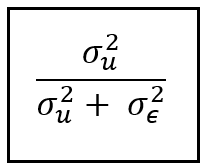
Estimation of σ²_ϵ and σ²_u also gives us a way to estimate the fraction of the total variance in y that the random effects model was able to explain, as follows:
The estimation procedure for the Random Effects model proceeds through the following sequence of steps:
STEP 1: Estimation of the Pooled OLSR regression model
The Random Effects model has the composite error term (μ + ϵ). In this step, we will prepare the ground for estimating the variances σ²_ϵ and σ²_u associated with components μ and ϵ. These variance estimates will be needed later on to estimate the model’s coefficients.
To that end, we will train a Pooled OLS regression model model on the panel data set. The Pooled OLSR model is basically an OLS regression model that is built on the flattened version of the panel data set.
In case of the World Bank data set, we regress GDP_PCAP_GWTH_PCNT on GCF_GWTH_PCNT:

What we are really interested in are the residual errors ϵ of the trained PLSR model. In the next step, we will use these errors for estimating the variance components of the Random Effects model.
STEP 2: Estimation of variance components σ²_ϵ and σ²_u
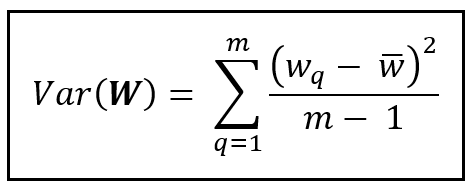
σ²_ ϵ and σ²_ μ are the variances of error components μ and ϵ. For estimating the variance, we will use the formula for sample variance:
It can be shown that the variance σ²_ ϵ is simply the variance of the error term ϵ of the Fixed Effects model. Therefore, to estimate this variance, we will train a Fixed Effects model on the panel data set as illustrated in my article on Fixed Effects models. Then, we use the residual errors from the fitted model to calculate σ²_ ϵ as follows:
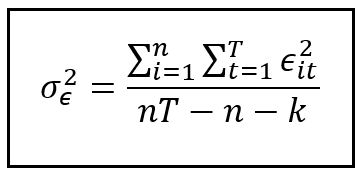
In the above formula, ϵ_i_t is the residual error for unit i at time t from the trained FE model. Notice that we have not de-meaned (i.e. subtracted the mean from) each error because the mean of the residual errors from a fitted OLSR model (which is what the FE model essentially is) is zero.
In the above formula, the inner summation is the sum of squares of the residual errors for unit i. The outer sum performs the inner summation across all n units in the data panel.
In the denominator, we have adjusted down the total degrees of freedom (nT) by the number of groups (n) and the number of regression variables (k) in each group that the Fixed Effects model uses.
The procedure for computing σ²_u which is the variance attributable to unit-specific effects is somewhat convoluted. There are at least three different formulae presented for it in the literature on panel data regression. We won’t go into the details and rationale for these formulae and instead simply state the one that is easiest to understand:

In the above formula, σ²_pooled is the variance of the residual errors of the Pooled OLSR model trained on the panel data set. Recollect that we fitted this model in STEP 1. We have already seen how to estimate σ²_ ϵ. Therefore, knowing σ²_pooled and σ²_ ϵ, we can use the above formula to estimate σ²_u.
In the next two steps, we will further prepare the ground for estimating the coefficients β and the common bias α.
STEP 3: Estimation of the group-specific means
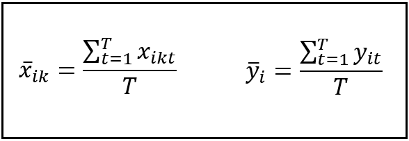
In this step, we will calculate the means of the response y_i and regression variables X_i for each group i (i.e. each unit i) in the data panel. Since our data panel is balanced, each group contains the same number of T time periods. So, calculation of the mean for group i involves taking the sum of all values of response value y for group i (or the sum of all values of regression variable x_k for group i) and dividing the sum by T, as follows:
The following figure illustrates this calculation for Belgium:

Many texts denote such means using the following notation:
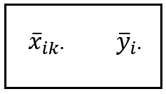
The location of the dot indicates the matrix dimension over which the aggregation is performed. In the above case, the aggregation is performed over the time dimension.
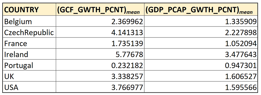
The following table contains the group-specific means for the WB data set:
Here’s how these values look like when plotted against each other:
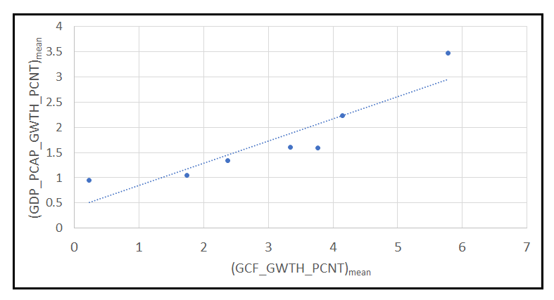
We will use these group-means in the next step.
STEP 4: Calculation of the centered (mean-subtracted) data panel
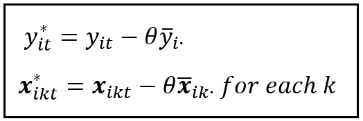
In this step, we de-mean all y_i and X_i values for each unit using the respective group-specific mean calculated in STEP 3. But instead of centering the data set around the raw group-specific mean, we center it around a scaled version of the mean where the scaling factor θ embodies the contribution of the unit-specific random effect. Here are the equations for centering the y_i and X_i values:
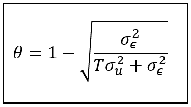
The scaling factor θ can be expressed in terms of the two variance components σ²_ϵ and σ²_u as follows:
STEP 5: Estimation of Random Effects model coefficients β_i using the mean-subtracted data panel
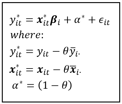
Finally, we estimate the coefficients β_i of the random effects model. We do that by fitting an OLSR model on the mean-subtracted data panel ( y*, X*) that we constructed in STEP 4. The model equations for unit i at time t are as follows:
This completes the estimation procedure for the Random Effects model.
How to implement the Random Effects regression model using Python and statsmodels
We will now illustrate the procedure for building and training the Random Effects regression model on the World Bank data set using the 5-step procedure that we outlined above.
At the beginning of the article, we had imported all the required packages and loaded the World Bank data set into a Pandas Dataframe.
Let’s lay out all that code include common variable definitions which we will use in later steps:
colors_master = ['blue', 'red', 'orange', 'lime', 'yellow', 'cyan', 'violet', 'yellow', 'sandybrown', 'silver']

#Define the units (countries) of interest
unit_names = ['Belgium', 'CzechRepublic', 'France', 'Ireland', 'Portugal', 'UK', 'USA']
unit_names.sort()

colors = colors_master[:len(unit_names)]

unit_col_name='COUNTRY'
time_period_col_name='YEAR'

#Define the y and X variable names
y_var_name = 'GDP_PCAP_GWTH_PCNT'
X_var_names = ['GCF_GWTH_PCNT']

#Load the panel data set of World Bank published development indicators into a Pandas Dataframe
df_panel = pd.read_csv('wb_data_panel_2ind_7units_1992_2014.csv', header=0)
#Setup the variables that we will use in later steps to calculate the variance components

#n=number of groups
n=len(unit_names)

#T=number of time periods per unit
T=df_panel.shape[0]/n

#N=total number of rows in the panel data set
N=n*T

#k=number of regression variables of the Pooled OLS model
k=len(X_var_names)+1
plot_against_X_index=0

#Use Seaborn to plot GDP growth over all time periods and across all countries versus gross
# capital formation growth:
sns.scatterplot(x=df_panel[X_var_names[plot_against_X_index]], y=df_panel[y_var_name], hue=df_panel[unit_col_name], palette=colors).set(title= 'Y-o-Y % Change in per-capita GDP versus Y-o-Y % Change in Gross capital formation')
plt.show()
The data set is available for download over here.
STEP 1: Estimate the Pooled OLSR regression model
In this step, using statsmodels, we will build and train a Pooled OLS regression model on the panel data set:
#Carve out the pooled y and pooled X matrices
grouped_y=df_panel_group_means[y_var_name]
grouped_X=df_panel_group_means[X_var_names]
#Add the placeholder for the regression intercept
grouped_X = sm.add_constant(grouped_X)
#Build and train an OLSR model on the entire dataset
pooled_olsr_model = sm.OLS(endog=pooled_y, exog=pooled_X)
pooled_olsr_model_results = pooled_olsr_model.fit()
print('=============== Pooled OLSR Model ===============')
print(pooled_olsr_model_results.summary())
We get the following output:
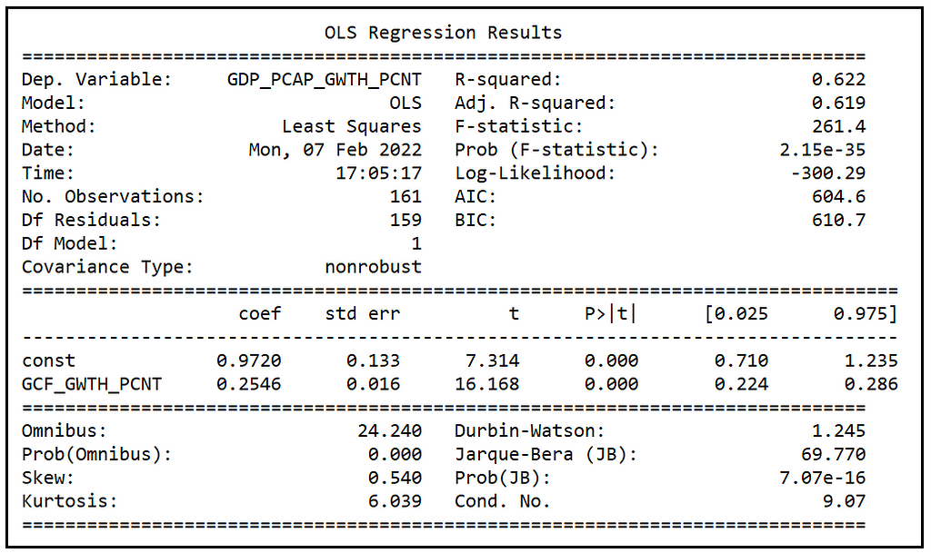
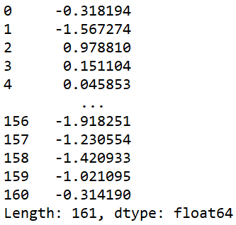
We are interested in the residual errors of this model which are as follows:
print('residuals of the \'Pooled OLSR\' model:')
print(pooled_olsr_model_results.resid)
STEP 2: Calculation of variance components σ²_ϵ and σ²_u
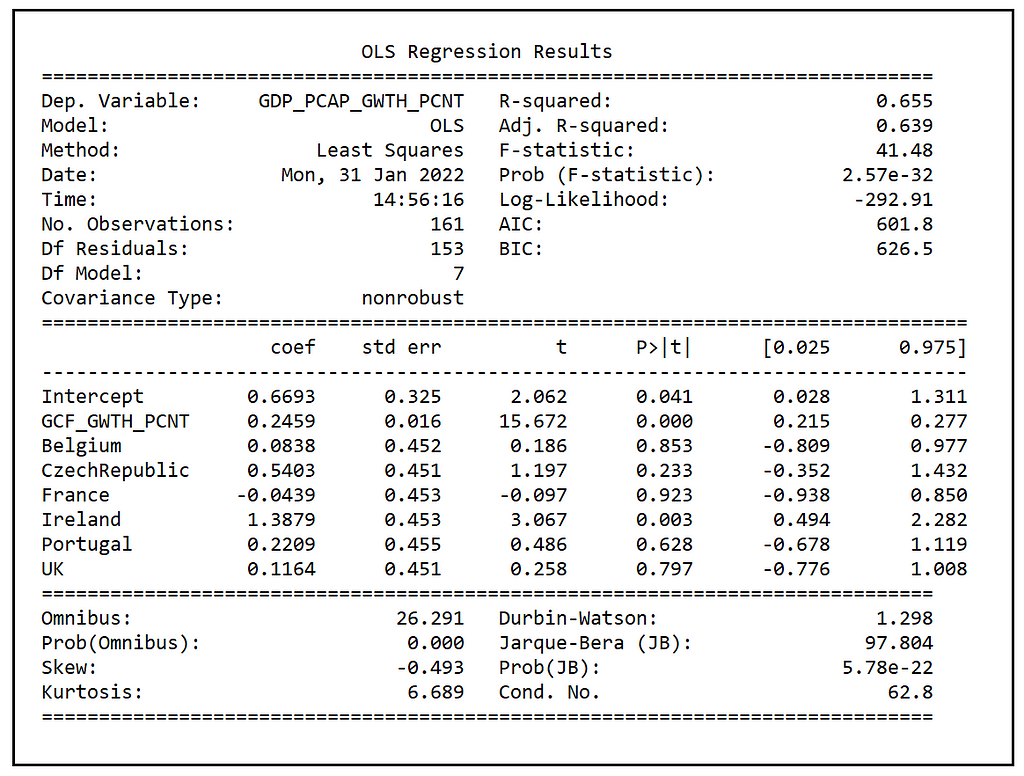
To calculate σ²_ϵ, we’ll fit the Fixed Effects model on this data set.
Build and fit an LSDV (Least Squares with Dummy Variables) model on the panel data set so that we can access it’s SSE.
Create the dummy variables, one for each country.
df_dummies = pd.get_dummies(df_panel[unit_col_name])
Join the dummies Dataframe with the panel data set.
df_panel_with_dummies = df_panel.join(df_dummies)
Construct the regression equation for the LSDV model. Note that we are leaving out one dummy variable so as to avoid perfect multicolinearity between the 7 dummy variables. The regression model’s intercept will contain the value of the coefficient for the omitted dummy variable for United States.
lsdv_expr = y_var_name + ' ~ '
i = 0
for X_var_name in X_var_names:
    if i > 0:
        lsdv_expr = lsdv_expr + ' + ' + X_var_name
    else:
        lsdv_expr = lsdv_expr + X_var_name
    i = i + 1
for dummy_name in unit_names[:-1]:
    lsdv_expr = lsdv_expr + ' + ' + dummy_name

print('Regression expression for OLS with dummies=' + lsdv_expr)
Build and train the LSDV model.
lsdv_model = smf.ols(formula=lsdv_expr, data=df_panel_with_dummies)
lsdv_model_results = lsdv_model.fit()
Print out the training summary.
print('============= OLSR With Dummies =============')
print(lsdv_model_results.summary())
We see the following output:
Calculate and print σ²_ϵ:
sigma2_epsilon = lsdv_model_results.ssr/(n*T-(n+k+1))
print('sigma2_epsilon = ' + str(sigma2_epsilon))
We get the following value for σ²_ϵ:
sigma2_epsilon = 2.359048222628497
Calculate σ²_pooled:
sigma2_pooled = pooled_olsr_model_results.ssr/(n*T-(k+1))
print('sigma2_pooled = ' + str(sigma2_pooled))
We get the following value for σ²_pooled:
sigma2_pooled = 2.4717633611733136
Calculate σ²_u:
sigma2_u = sigma2_pooled - sigma2_epsilon
print('sigma2_u = ' + str(sigma2_u))
We get the following value:
sigma2_u = 0.11271513854481663
STEP 3: Estimate the group-specific means
Calculate the means of the y_i and X_i values for each group (i.e. each unit i) in the data panel as follows:
df_panel_group_means = df_panel.groupby(unit_col_name).mean()
print(df_panel_group_means)
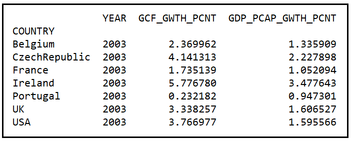
The YEAR column can be ignored in the above grouped data panel.
Let’s append a column for storing the regression intercept to this Dataframe. We’ll use that column in STEP 5 for estimating the common bias α:
df_panel_group_means['const'] = 1.0
STEP 4: Calculate the centered (mean-subtracted) data panel
In this step, we will de-mean all y_i and X_i values for each unit, using the scaled version of the respective group-specific mean calculated in STEP 2.
Let’s calculate θ:
theta = 1 - math.sqrt(sigma2_epsilon/(sigma2_epsilon + T*sigma2_u))
print('theta = ' + str(theta))
We get the following value:
theta = 0.30975991786766044
Prepare the data set for mean centering the y and X columns:
pooled_y_with_unit_name = pd.concat([df_panel[unit_col_name], pooled_y], axis=1)
pooled_X_with_unit_name = pd.concat([df_panel[unit_col_name], pooled_X], axis=1)
Center each X value using the θ-scaled group-specific mean:
unit_name = ''
for row_index, row in pooled_X_with_unit_name.iterrows():
    for column_name, cell_value in row.items():
        if column_name == unit_col_name:
            unit_name =
                pooled_X_with_unit_name.at[row_index, column_name]
        else:
            pooled_X_group_mean =
                df_panel_group_means.loc[unit_name][column_name]
            pooled_X_with_unit_name.at[row_index, column_name] =
                pooled_X_with_unit_name.at[
                row_index, column_name] - theta*pooled_X_group_mean
Center each y value using the θ-scaled group-specific mean:
unit_name = ''
for row_index, row in pooled_y_with_unit_name.iterrows():
    for column_name, cell_value in row.items():
        if column_name == unit_col_name:
            unit_name =
                pooled_y_with_unit_name.at[row_index, column_name]
        else:
            pooled_y_group_mean =
                df_panel_group_means.loc[unit_name][column_name]
            pooled_y_with_unit_name.at[row_index, column_name] =
                pooled_y_with_unit_name.at[
                row_index, column_name] - theta*pooled_y_group_mean
STEP 5: Estimate Random Effects model coefficients β_i using the mean-subtracted data panel
Finally, let’s build and train the RE model on the pooled_X_with_unit_name and pooled_X_with_unit_name.
Carve out the y and X matrices:
re_y=pooled_y_with_unit_name[list(pooled_y_with_unit_name.columns[1:])]
re_X=pooled_X_with_unit_name[list(pooled_X_with_unit_name.columns[1:])]
Build and train an OLS regression model:
re_model = sm.OLS(endog=re_y, exog=re_X)
re_model_results = re_model.fit()
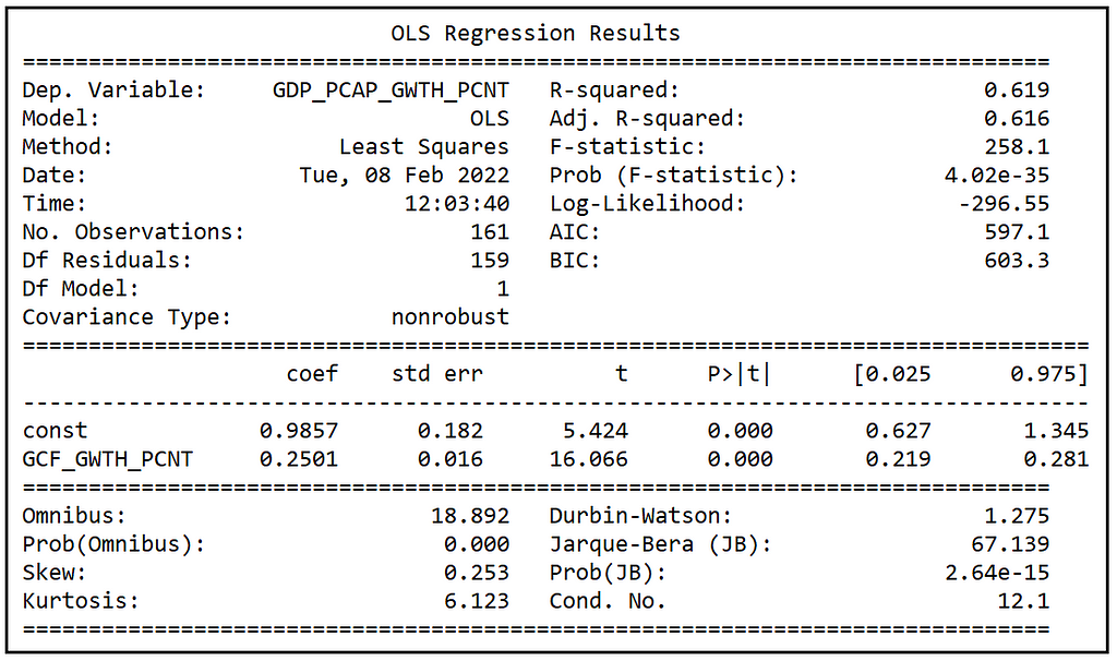
Print the training summary:
print(re_model_results.summary())
We see the following output:
This completes the estimation procedure of the Random Effects regression model.
Testing the significance of the Random Effect
Recollect that σ²_u was estimated to 0.112723 and σ²_ϵ was estimated to be 2.35905. So the fraction of the total variance that can be attributable to unit-specific random effect is:
0.112723/(0.112723+2.35905)=0.04560 i.e. about 4%.
The small size of the random effect gives provides the first hint that the Random Effects model may not be suitable for this data set, and a Fixed Effects model may turn out to provide a better fit.
We can use the Breusch-Pagan LM Test for testing the significance of the Random Effect.
The null hypothesis of the Breusch-Pagan LM test is that the unit-specific variance σ²_u is zero.
The test statistic is as follows:

Under the null hypothesis of the LM test, the test statistic is Chi-squared(1) distributed.
The nested-summation in the denominator is the sum of squares of residuals from the Pooled OLSR model which we fitted in STEP 1. The summation in the numerator is the sum of the group-wise means of the residual errors from the Pooled OLSR model. Notice the bar over the ϵ which indicates that it is the mean residual error , and the ‘dot’ after the ‘i’ subscript which indicates that the mean is over the set of all time periods in each group. There are n groups corresponding to n units in the data panel. Hence the summation in the numerator goes from 1 through n.
Let’s compute the value of this statistic for the World Bank data set:
#Concatenate the unit names column to the Dataframe containing the residuals from the Pooled OLSR model
df_pooled_olsr_resid_with_unitnames = pd.concat([df_panel[unit_col_name],pooled_olsr_model_results.resid], axis=1)
df_pooled_olsr_resid_group_means = df_pooled_olsr_resid_with_unitnames.groupby(unit_col_name).mean()
ssr_grouped_means=(df_pooled_olsr_resid_group_means[0]**2).sum()
ssr_pooled_olsr=pooled_olsr_model_results.ssr
LM_statistic = (n*T)/(2*(T-1))*math.pow(((T*T*ssr_grouped_means)/ssr_pooled_olsr - 1),2)

print('BP LM Statistic='+str(LM_statistic))
We see the following output:
LM Statistic=3.4625558219208075
Let’s print out the critical Chi-squared(1) value at an α=.05:
alpha=0.05
chi2_critical_value=st.chi2.ppf((1.0-alpha), 1)
print('chi2_critical_value='+str(chi2_critical_value))
We see the following output:
chi2_critical_value=3.841458820694124
The test statistic of the LM test (3.46256) is less than the Chi-squared(1) critical value of 3.84146 at α=.05, which means the random effect is not significant at an alpha of .05. (Don’t confuse this α with the one symbolizing the mean unit-specific effect of the RE model!)
Performance comparison of the Pooled OLSR, the Fixed Effects, and the Random Effects models
It would be useful to compare the performance of the three models on the WB data set. For the Pooled OLSR and the FE models, we’ll draw upon the results obtained for those models from the respective articles.
Comparison of coefficients
We find that the coefficient of the GCF_GWTH_PCNT regression variable estimated by the three models is approximately the same:

Comparison of goodness-of-fit measures

We see that in the Fixed Effects model, the adjusted R-squared (which is R-squared after accounting for the reduction in degrees of freedom due to inclusion of regression variables), is marginally improved from 0.619 to 0.639 over the Pooled OLSR model, while the Random Effects model produces almost no improvement in adj. R-squared over the Pooled OLSR model.
The FE model also produces a small increase in the Log-likelihood from -300.29 to -292.91 over the Pooled model, and a corresponding small improvement (reduction) in the AIC score from 604.6 to 601.8 over the Pooled OLSR model. The RE model produces a further improvement of the AIC score to 597.1 over the FE model.
The FE model can be seen to produce an overall improvement in the goodness-of-fit (albeit by a small margin) over that of the Pooled model, while the same cannot be said about the Random model’s performance. This is further evidenced by the tiny (4%) contribution of random effect in the variance of the error term and its insignificance established by the LM test.
Here is the complete source code used in this article:
References, Citations and Copyrights
Data set
World Development Indicators data from World Bank under CC BY 4.0 license. Download link
Paper and Book Links
The following two books pretty much cover the field of Panel Data Analysis and most practitioners need look no further:
Badi H. Baltagi, Econometric Analysis of Panel Data, 6th Edition, Springer
William H. Greene, Econometric Analysis, 8th Edition, 2018, Pearson
If you are a Stata user, you may find the following introduction to the field and tutorials from Hun Myoung Park quite informative: Practical Guides To Panel Data Modeling: A Step by Step Analysis Using Stata
Images
All images in this article are copyright Sachin Date under CC-BY-NC-SA, unless a different source and copyright are mentioned underneath the image.
The No-Nonsense Guide to the Random Effects Regression Model was originally published in Towards Data Science on Medium, where people are continuing the conversation by highlighting and responding to this story.
from Towards Data Science - Medium https://ift.tt/9ElWs8C
via RiYo Analytics

No comments