https://ift.tt/YRbVCDa ITS is one of the strongest quasi-experimental designs. Properly planning for the study is arguably more important t...
ITS is one of the strongest quasi-experimental designs. Properly planning for the study is arguably more important than the analysis itself.

Why Interrupted Time Series design?
Evidence-based practice is the basis of modern medicine. In order for machine learning (ML) models to be integrated into clinical care, we need to be able to attribute the observed effects in health outcomes and/or operational efficiency to the models with a high level of confidence.
Predictive ML models have largely been developed based on observational data. However, it is misleading to draw causal relationships from these observational studies. They can generate hypotheses for further testing but are rarely useful to evaluate the effectiveness of our models in real world.
Randomized control trial (RCT) is considered the gold standard method of assessing healthcare innovations. However, in many cases, RCT is not possible due to practical or ethical barriers. The Interrupted Time Series (ITS) design is a possible alternative, and is in fact one of the strongest quasi-experimental designs.
What is Interrupted Time Series Design?
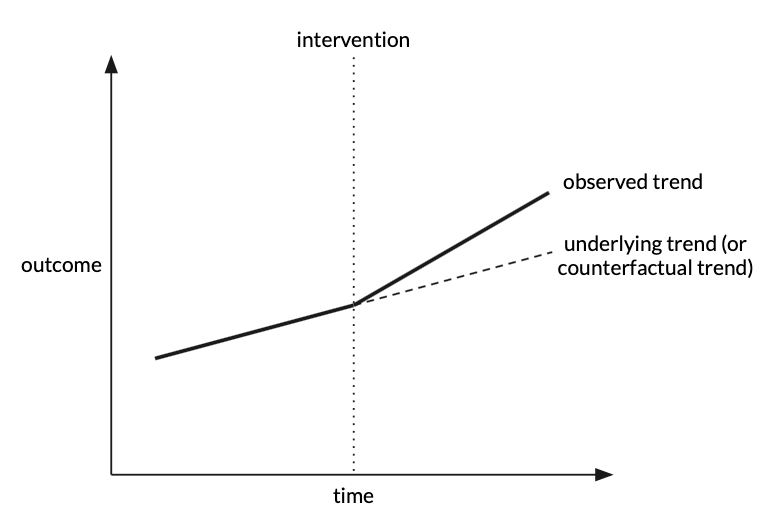
In ITS, the effects of an intervention (e.g. deployed ML model) are evaluated by comparing outcome measures obtained at several time points before and several time points after the intervention is introduced. The goal is to detect whether the intervention has had an effect greater than the underlying trend.
Power & Sample Size Planning for ITS
Planning how the ITS should be carried out is crucial, and arguably even more important than the analysis. A badly designed study can never be retrieved, whereas a poorly analyzed one can be reanalyzed. How the study is designed also governs how the data is to be analyzed. To ensure validity and adequate power for the study, we need to carefully plan how big the sample size should be, which is also closely related to how long the study should last and how frequently we should collect data. There’s no exact formula to calculate the minimum sample size required for ITS. Instead, there are various factors need to be collectively considered:
- Number of time points in each before- and after- segment
- Average sample size per time point
- Frequency of time points (i.e. weekly, monthly, yearly, etc.)
- Location of intervention (i.e. midway, 1/3, 2/3, etc.)
- Expected effect size
Number of time points before- and after-
ITS relies on repeated observations of an outcome event over time, usually at equally spaced intervals. Here, we refer to an observation of outcome event as a time point in the time series analysis. There are usually two segments in a ITS design: a before-intervention segment and an after-intervention segment.
There are conflicting recommendations as to the minimum number of time points needed. Recommendations range from 3 time points per segment to 50 time points per segment. Many papers which conduct systematic review of ITS do not even consider studies with fewer than 3 time points per segment due to their questionable validity.
Depending on the methods used to analyze the trends in time series, different number of time points are required. For example, if use Ordinary Least Squares (OLS), 50 time points overall can be considered a long time series, but if use ARIMA, 50 time points is the minimum. Overall, the fewer time points available, the simpler correlation structures can be reliably estimated.
Although there’s no gold standard in the minimum number of time points required, the general consensus is that longer time series tend to have more power than shorter time series.
Sample size per time point
Even for a time series with many time points, if only a small number of subjects constitutes the estimate for a time point of outcome event, it’s improbable to detect a true effect due to noise and variability. A larger number of subjects constituting each time point provides more stable estimates and thus reduces the variability and outliers within a time series analysis.
Frequency of time points
There is a trade-off between number of time points and sample size per time point, depending on the choice of time interval. To optimize the study power, you can sacrifice sample size per time point to increase the total number of time points, or vice versa. For example, on average, there are 10 distinct subjects per week that can be used to calculate the outcome measure. You can only afford to run the study for 6 months. If you choose frequency of time points to be monthly, the time series will consist of 6 time points where sample size per time point is 40. If you choose frequency to be bi-weekly, there will be 12 time points in total and sample size per time point is 20. In most cases, only very little gain in power is achieved when a time series is lengthened at the expense of sample size per time point. When a very short time series is lengthened, gains are more noticeable.
When possible, choose frequency that have clinical or seasonal meaning so that a true underlying trend can be established. Also consider whether there may be a delay or waning intervention effect, especially when the impact occurs gradually, so you can choose frequency accordingly.
Location of intervention
You can plan to introduce your intervention midway of the time series (most common scenario), early in the time series (e.g. 1/3 of time points are before intervention) or later in the time series (e.g. 2/3 of time points are before intervention). As long as there are sufficient time points per segment and each time point is supported by a large enough sample size, there is not much difference in the study power of an early or late intervention, as compared to when the intervention occur midway through.
Expected effect size
Before setting out to implement your study, you should hypothesize how the intervention would impact on the outcome if it were effective. In ITS, there are two main types of effects:
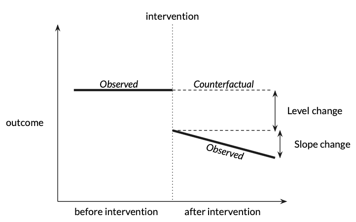
- Slope change: a gradual change in gradient (or slope) of trend
- Level change: an instant change in level
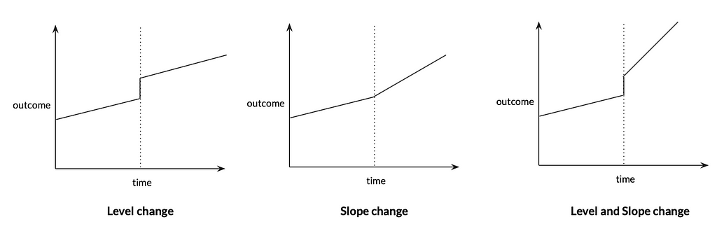
These two effects do not need to be mutually exclusive. You can have a level change, a slope change, or a level and slope change. These changes can also be temporary or have a lagging property.
Effect size is the magnitude of intervention effect. It is generally easier to detect a large effect size than a small one. In other words, when the expected effect size is large, we need fewer time points and smaller sample size per time point to ensure adequate power.
As you may have noticed by now, this article does not provide any straightforward sample size formula for ITS (sorry!) because there is none. Researchers and data scientists should consider multiple factors according to their specific scenarios. Those factors presented in the article are the minimum set of requirements that would inform the planning process of ITS design.
Sample Size Planning for Interrupted Time Series Design in Health Care was originally published in Towards Data Science on Medium, where people are continuing the conversation by highlighting and responding to this story.
from Towards Data Science - Medium https://ift.tt/zuBD18j
via RiYo Analytics


No comments