https://ift.tt/Zxf8Oat It’s all about the features Image on Unsplash by Sébastien Lavalaye When we think about boosted trees in the ti...
It’s all about the features

When we think about boosted trees in the time series space, it is usually in regards to the M5 competition where a significant portion of the top ten entries were using LightGBM. However, when looking at the performance of boosted trees in the univariate case, where there is not a wealth of exogenous features to utilize, their performance has been…rough.
Until now.
Section 1: The Intro
First, I should throw in some caveats. The runner-up in the M4 competition DID use boosted trees. However, it was as a meta-model to ensemble other, more traditional, time series methods. All benchmarking I have seen on M4 with more standard boosted trees have been fairly abysmal, sometimes not even competing with naïve forecasters. The main resource I use here comes from the excellent work done for the Sktime package and their paper[1]:
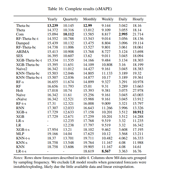
Any model with ‘XGB’ or ‘RF’ is using a tree-based ensemble. We do see one example where Xgboost provides the best result in the hourly dataset with a 10.9! Then, we realize these are only the models they tried in their framework and the winner of M4 posted a 9.3 for the same dataset…
Try to remember some of the numbers from this chart for later, specifically the 10.9 for the hourly dataset from XGB-s and the ‘best’ results for trees in the weekly dataset: 9.0 from RF-t-s.
Our goal is to absolutely crush these numbers with a fast LightGBM procedure that fits individual time series and is comparable to stat methods in terms of speed.
So, no time for optimization.
Sounds pretty difficult, and our first thought may be that we have to optimize our trees. Boosted trees are so complicated and we are fitting individual data sets so they must have different parameters.
But it’s all about the features.
Section 2: The Features
When looking at other implementations for trees in the univariate space you will see some feature engineering such as binning, using lagged values of your target, a simple counter, seasonal dummies, and maybe Fourier basis functions here and there. All of this is great if you want to regret fitting boosted trees and wish that you instead stuck with an exponential smoother. The theme is that we have to featurize our time element and represent it as tabular data to feed to the tree, and our implementation: LazyProphet, is no exception. But, we have one extra element of feature engineering that I have not seen anywhere (although it’s quite simple so there is no way this is novel).
We will…‘connect the dots’.
Quite simply, we connect the first point of our series and fit a line to another point midway through, then connect that point to the final point. Repeat that a couple of times while changing which point to use as a the “kink” and you are in business.
Hopefully this graph illustrates it well. The blue line is a time series and the other lines are just ‘connecting the dots’:
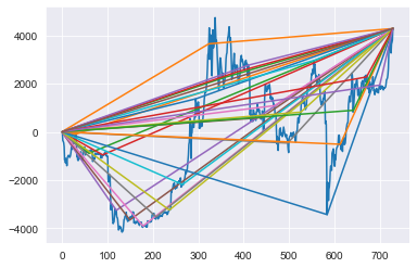
It turns out, these are just weighted piecewise linear basis functions. (Once again, if you know of any research on this definitely let me know as I can’t really find anything on this specific implementation.) One downside of this is that there can be wonkiness in the extrapolation of these lines. To handle this, we will throw on a ‘decay’ factor which simply penalizes the slope of each line from the mid-point to the final point.
There you go, that’s it. Throw in some of these bad boys along with lagged target values and Fourier basis functions and you’ve done it! Near state-of-the-art performance for certain problems and there is very little that is required from us, thus the name ‘LazyProphet’.
But let’s get some results to back this up.
Section 3: The Code
The datasets are all open source and live on the M-competitions github. It is split up by the standard train and test splits, so we will use the train csv for fitting and the test csv only for evaluation using the SMAPE. Let’s go ahead and import the data along with LazyProphet, if you haven’t installed it yet go ahead and grab it from pip.
pip install LazyProphet
After installing, let’s get to coding:
import matplotlib.pyplot as plt
import numpy as np
from tqdm import tqdm
import pandas as pd
from LazyProphet  import LazyProphet as lp
train_df = pd.read_csv(r'm4-weekly-train.csv')
test_df = pd.read_csv(r'm4-weekly-test.csv')
train_df.index = train_df['V1']
train_df = train_df.drop('V1', axis = 1)
test_df.index = test_df['V1']
test_df = test_df.drop('V1', axis = 1)
Here we just import all the necessary packages and read in the data as standard DataFrames for the weekly data. Next, let’s create our SMAPE function which will return the SMAPE given forecasts and actuals:
def smape(A, F):
    return 100/len(A) * np.sum(2 * np.abs(F - A) / (np.abs(A) +       np.abs(F)))
For our experiment we will take the average across all time series to compare against other models. For a sanity check, we will also get the ‘naïve’ average SMAPE to ensure what we are doing is consistent with what was done in the competition. With that said, we will simply iterate through the dataframe and lazily fit and predict. The code could be optimized by not doing a for-loop, but this will do fine!
smapes = []
naive_smape = []
j = tqdm(range(len(train_df)))
for row in j:
    y = train_df.iloc[row, :].dropna()
    y_test = test_df.iloc[row, :].dropna()
    j.set_description(f'{np.mean(smapes)}, {np.mean(naive_smape)}')
    lp_model = LazyProphet(scale=True,
                            seasonal_period=52,
                            n_basis=10,
                            fourier_order=10,
                            ar=list(range(1, 53)),
                            decay=.99,
                            linear_trend=None,
                            decay_average=False)
    fitted = lp_model.fit(y)
    predictions = lp_model.predict(len(y_test)).reshape(-1)
    smapes.append(smape(y_test.values,      pd.Series(predictions).clip(lower=0)))
    naive_smape.append(smape(y_test.values, np.tile(y.iloc[-1], len(y_test))))
print(np.mean(smapes))
print(np.mean(naive_smape))
Before we look at the results let’s take a quick look at the LazyProphet parameters.
- scale: This one is easy, simply whether or not to scale the data. The default is True so we are just being explicit here.
- seasonal_period: This parameter controls the Fourier basis functions for the seasonality, since this is weekly frequency we use 52.
- n_basis: This parameter controls our patent-pending weighted piecewise linear basis functions. This is just an integer for the number of functions to use.
- fourier_order: The number of sine and cosine pairs to use for seasonality.
- ar: What lagged target variable values to use. Can take a list for multiple and we simply pass a list of 1–52.
- decay: Our decay factor used for penalizing the ‘right’ side of our basis functions. Setting to 0.99 means the slope is multiplied by (1- 0.99) or 0.01.
- linear_trend: One major downside of trees is that they cannot extrapolate out of the bounds of previous data. Did I mention that yet? Yeah, that can be a huge issue. To overcome this, there are some off-the-cuff tests for a polynomial trend and if one is detected we fit a linear regression to de-trend. Passing None denotes there will be tests, passing True denotes ALWAYS detrending, and passing False denotes to NOT test and never use a linear trend.
- decay_average: Not a useful parameter when using a decay rate. This is mostly weird dark magic that does weird things. Try it out! But don’t use it. Passing True essentially just averages all the future values of the basis function. This was useful when fitting with an elasticnet procedure but less useful with LightGBM in my testing.
Before we get to the results, let’s go ahead and fit on the hourly dataset as well:
train_df = pd.read_csv(r'm4-hourly-train.csv')
test_df = pd.read_csv(r'm4-hourly-test.csv')
train_df.index = train_df['V1']
train_df = train_df.drop('V1', axis = 1)
test_df.index = test_df['V1']
test_df = test_df.drop('V1', axis = 1)
smapes = []
naive_smape = []
j = tqdm(range(len(train_df)))
for row in j:
    y = train_df.iloc[row, :].dropna()
    y_test = test_df.iloc[row, :].dropna()
    j.set_description(f'{np.mean(smapes)}, {np.mean(naive_smape)}')
    lp_model = LazyProphet(seasonal_period=[24,168],
                            n_basis=10,
                            fourier_order=10,
                            ar=list(range(1, 25)),
                            decay=.99)
    fitted = lp_model.fit(y)
    predictions = lp_model.predict(len(y_test)).reshape(-1)
    smapes.append(smape(y_test.values, pd.Series(predictions).clip(lower=0)))
    naive_smape.append(smape(y_test.values, np.tile(y.iloc[-1], len(y_test))))
print(np.mean(smapes))
print(np.mean(naive_smape))
Alright, all we really changed was the seasonal_period and the ar arguments. When passing a list to seasonal_period it will build out the seasonal basis functions for everything in the list. ar was adjusted to fit the new major seasonal period of 24. That’s it!
Section 4: The Results
Remember the Sktime results from above? You actually don’t have to, here is a table:
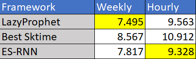
So, LazyProphet beat out the best of Sktime’s models, which included several different tree-based methods. We did lose to the winner of M4 on the hourly dataset, but on average we actually outperform ES-RNN overall. The important thing to realize here is that we did this with default parameters…
boosting_params = {
                    "objective": "regression",
                    "metric": "rmse",
                    "verbosity": -1,
                    "boosting_type": "gbdt",
                    "seed": 42,
                    'linear_tree': False,
                    'learning_rate': .15,
                    'min_child_samples': 5,
                    'num_leaves': 31,
                    'num_iterations': 50
                    }
If you want to change these you could just pass your own dict when creating the LazyProphet class. These could even be optimized for each time series for even more gains.
But, let’s compare our results with our goals:
- We did zero parameter optimization (with slight modifications for different seasonalities).
- We fit each time series individually.
- We produced the forecasts ‘lazily’ in just over a minute on my local machine.
- We beat every other tree method from our benchmark, heck, we even beat the winner of M4 on average.
I’d say we were pretty successful!
You may be asking, “Where are the results of the other datasets?”
Unfortunately, our success wasn’t long lasting. The other datasets, generally, had way less data so our method tended to have significantly degraded performance. From what I can tell, LazyProphet tends to shine with high frequency and a decent amount of data. Of course, we could try fitting all of the time series with a single LightGBM model but we can save that for next time!
Since we are just using LightGBM, you can alter the objective and try out time series classification! Or use a quantile objective for prediction bounds! Lot’s of cool things to try out.
If you found this interesting I encourage you to check out my other look at the M4 competition with another home-grown method: ThymeBoost.
- The M4 Time Series Forecasting Competition with ThymeBoost
- Time Series Forecasting with ThymeBoost
- Gradient Boosted ARIMA for Time Series Forecasting
References:
LazyProphet: Time Series Forecasting with LightGBM was originally published in Towards Data Science on Medium, where people are continuing the conversation by highlighting and responding to this story.
from Towards Data Science - Medium https://ift.tt/SOWRKGl
via RiYo Analytics


No comments