https://ift.tt/RCW7nOv Learn how the gradient descent algorithm works by implementing it in code from scratch. Image by Author (created u...
Learn how the gradient descent algorithm works by implementing it in code from scratch.
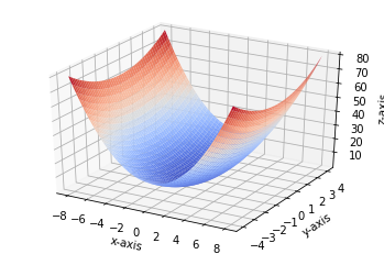
A machine learning model may have several features, but some feature might have a higher impact on the output than others. For example, if a model is predicting apartment prices, the locality of the apartment might have a higher impact on the output than the number of floors the apartment building has. Hence, we come up with the concept of weights. Each feature is associated with a weight (a number) i.e. the higher the feature has an impact on the output, the larger the weight associated with it. But how do you decide what weight should be assigned to each feature? This is where gradient descent comes in.
Gradient Descent is an optimisation algorithm which helps you find the optimal weights for your model. It does it by trying various weights and finding the weights which fit the models best i.e. minimises the cost function. Cost function can be defined as the difference between the actual output and the predicted output. Hence, the smaller the cost function is, the closer the predicted output from your model is to the actual output. Cost function can be mathematically defined as:
𝑦=𝛽+θnXn,
where x is the parameters(can go from 1 to n), 𝛽 is the             bias and θ is the weight
While on the other hand, the learning rate of the gradient descent is represented as α. Learning rate is the size of step taken by each gradient. While a large learning rate can give us poorly optimised values for 𝛽 and θ, the learning rate can also be too small which takes a substantial increment in number of iterations required to get the the convergence point(the optimal value point for 𝛽 and θ). This algorithm, gives us the value of α, 𝛽 and θ as output.
If you want to understand gradient descent and cost functions more in detail, I would recommend this article.
So now that we know what a gradient descent is and how it works, let’s start implementing the same in python. But, before we get to the code logic of the same, let’s first take a look at the data we are going to be using and the libraries that we will be importing for our purpose.
For this implementation, we are going to use the advertising dataset. This is a dataset that gives us the total sales for different products, after marketing them on Television, Radio and Newspaper. Using our algorithm, we can find out which medium performs the best for our sales and assign weights to all the mediums accordingly. This dataset can be downloaded from the link given below:
https://www.kaggle.com/sazid28/advertising.csv
Moving on to the imports, we will be using the libraries pandas and numpy, which will be used to read the data as well as perform mathematical functions on it. We will also be using matplotlib and seaborn to plot our findings and explain the results graphically. Once we have imported the libraries we will use pandas to read our dataset, and print the top 5 columns to reassure that the data has been read correctly. Once we have read the data, we will set the X & Y variables for our gradient descent curve.
import pandas as pd
import numpy as np
import matplotlib.pyplot as plt
import seaborn as sn
df=pd.read_csv('Advertising.csv')
df.head()
Output:
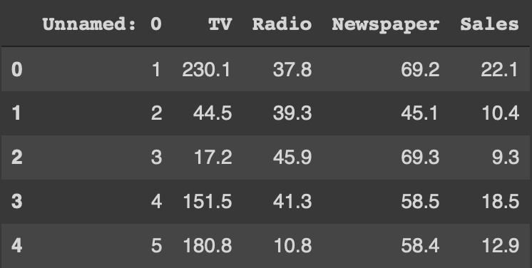
X would represent TV, Radio and Newspaper while Y would represent our sales. As all these sales might be on different scales, we then normalise our X & Y variables.
X=df[[‘TV’,’Radio’,’Newspaper’]]
Y=df[‘Sales’]
Y=np.array((Y-Y.mean())/Y.std())
X=X.apply(lambda rec:(rec-rec.mean())/rec.std(),axis=0)
Once we have a normalised dataset, we can start defining our algorithm. To implement a gradient descent algorithm we need to follow 4 steps:
- Randomly initialize the bias and the weight theta
- Calculate predicted value of y that is Y given the bias and the weight
- Calculate the cost function from predicted and actual values of Y
- Calculate gradient and the weights
To start, we will take a random value for bias and weights, which might be actually close to the optimal bias and weights or can be far off.
import random
def initialize(dim):
b=random.random()
theta=np.random.rand(dim)
return b,theta
b,theta=initialize(3)
print(“Bias: “,b,”Weights: “,theta)
Output:
Bias: 0.4439513186463464 Weights: [0.92396489 0.05155633 0.06354297]
Here, we have created a function named initialise which gives us some random values for bias and weights. We use the library random to give us the random numbers which fits to our needs. The next step is to calculate the output (Y) using these weights and bias.
def predict_Y(b,theta,X):
return b + np.dot(X,theta)
Y_hat=predict_Y(b,theta,X)
Y_hat[0:10]
Output:
array([ 3.53610908, 0.53826004, 1.4045012 , 2.27511933, 2.25046604, 1.6023777 , -0.36009639, -0.37804669, -2.20360351, 0.69993066])
Y_hat is the predicted output value whereas Y will be the actual value. The difference between these will give us our cost function. Which will be calculate in our next function.
import math
def get_cost(Y,Y_hat):
Y_resd=Y-Y_hat
return np.sum(np.dot(Y_resd.T,Y_resd))/len(Y-Y_resd)
Y_hat=predict_Y(b,theta,X)
get_cost(Y,Y_hat)
Output:
0.5253558445651124
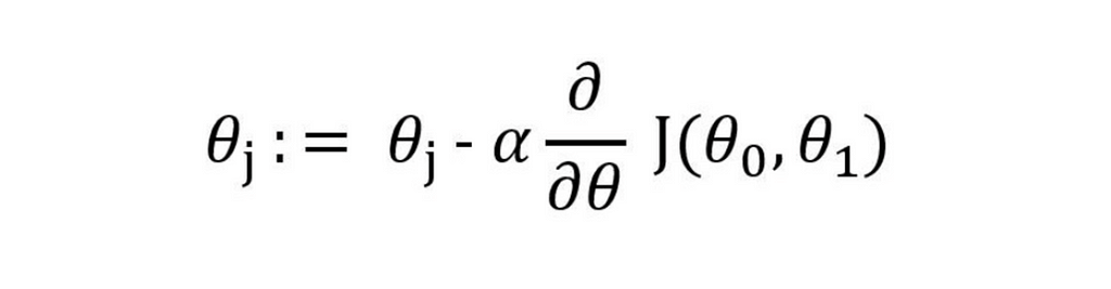
This is our cost function, and our aim is to reduce this as much as possible to get the most accurate predictions. To get the updated bias and weights we use the gradient descent formula of:
The parameters passed to the function are
- x,y : the input and output variable
- y_hat: predicted value with current bias and weights
- b_0,theta_0: current bias and weights
- Learning rate: learning rate to adjust the update step
def update_theta(x,y,y_hat,b_0,theta_o,learning_rate):
db=(np.sum(y_hat-y)*2)/len(y)
dw=(np.dot((y_hat-y),x)*2)/len(y)
b_1=b_0-learning_rate*db
theta_1=theta_o-learning_rate*dw
return b_1,theta_1
print("After initialization -Bias: ",b,"theta: ",theta)
Y_hat=predict_Y(b,theta,X)
b,theta=update_theta(X,Y,Y_hat,b,theta,0.01)
print("After first update -Bias: ",b,"theta: ",theta)
get_cost(Y,Y_hat)
Output:
After initialization -Bias:  0.4733071000028529 theta:  [0.56745402 0.43024717 0.0722811 ]
After first update -Bias:  0.46384095800279584 theta:  [0.57117721 0.43202382 0.07171437]
0.37245638135702513
As we can see, the cost function has reduced with the new bias and weights. Currently we are taking the learning rate as 0.001, we will also try with 0.01 to see if it can be a better and more optimal learning rate.
Now that we have created all the required functions we can create a main gradient descent function, which runs them for a particular number of iteration and finds us optimal bias and weights. For this implementation, we are running the function for 200 iterations.
def run_gradient_descent(X,
Y,
alpha,
num_iterations):
b,theta=initialize(X.shape[1])
iter_num=0
gd_iterations_df=pd.DataFrame(columns=[‘iteration’,’cost’])
result_idx=0
for each_iter in range(num_iterations):
Y_hat=predict_Y(b,theta,X)
this_cost=get_cost(Y,Y_hat)
prev_b=b
prev_theta=theta
b,theta=update_theta(X,Y,Y_hat,prev_b,prev_theta,alpha)
if(iter_num%10==0):
gd_iterations_df.loc[result_idx]=[iter_num,this_cost]
result_idx=result_idx+1
iter_num +=1
print(“Final Estimate of b and theta : “,b,theta)
return gd_iterations_df,b,theta
gd_iterations_df,b,theta=run_gradient_descent(X,Y,alpha=0.001,num_iterations=200)
Output:
Final Estimate of b and theta : 0.31516040347417285 [0.39731522 0.31571747 0.61334115]
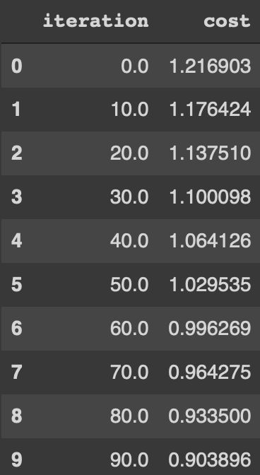
The theta comes as a list of 3 numbers, as we have 3 inputs, TV, radio and newspapers.If we print the cost function for each iteration we can see the decrease in the cost function. We can also plot the cost function to iterations to see the result.
gd_iterations_df[0:10]
Output:
%matplotlib inline
plt.plot(gd_iterations_df[‘iteration’],gd_iterations_df[‘cost’])
plt.xlabel(“Number of iterations”)
plt.ylabel(“Cost or MSE”)
Output:
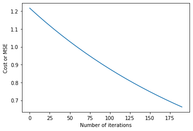
As we can see the cost function decreases with increase in iterations, but we still have not reached convergence. Now, let’s try with α=0.01 for 2000 iterations and compare it with α=0.001 and find which learning rate is better for this dataset.
alpha_df_1,b,theta=run_gradient_descent(X,Y,alpha=0.01,num_iterations=2000)
alpha_df_2,b,theta=run_gradient_descent(X,Y,alpha=0.001,num_iterations=2000)
plt.plot(alpha_df_1[‘iteration’],alpha_df_1[‘cost’],label=”alpha=0.01")
plt.plot(alpha_df_2[‘iteration’],alpha_df_2[‘cost’],label=”alpha=0.001")
plt.legend()
plt.ylabel(‘cost’)
plt.xlabel(‘Number of iterations’)
plt.title(‘Cost Vs. Iterations for different alpha values’)
Output:
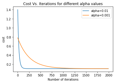
As one can see, 0.01 is the more optimal learning rate as it converges much quicker than 0.001. 0.01 converges around the 100 mark, while 0.001 takes 1000 iterations to reach convergence.
Hence, we have successfully built a gradient descent algorithm on python. Remember, the optimal value of learning rate will be different for each and every dataset.
Hope you learned something new and meaningful today.
Thank you.
Implementing Gradient Descent in Python from Scratch was originally published in Towards Data Science on Medium, where people are continuing the conversation by highlighting and responding to this story.
from Towards Data Science - Medium https://ift.tt/Nnt5sKf
via RiYo Analytics


No comments