https://ift.tt/BiMNLQ6 The Curse of Dimensionality A series of blog posts that summarize the Geometric Deep Learning (GDL) Course , at AM...
The Curse of Dimensionality
A series of blog posts that summarize the Geometric Deep Learning (GDL) Course, at AMMI program; African Master’s of Machine Intelligence, taught by Michael Bronstein, Joan Bruna, Taco Cohen, and Petar Veličković.
One of the most important needs in solving real-world problems is learning in high dimensions. As the dimension of the input data increases, the learning task will become more difficult, due to some computational and statistical issues. In this post, we discuss three stories in high-dimensional learning. First, we review some of the basics in statistical learning tasks. Then, we present the curse of dimensionality, how it occurs and affects learning. Finally, we introduce the geometric domains and their assumptions on the input data.
This post was co-authored with MohammedElfatih Salah. See also our last post on the Erlangen Programme of ML. Our main references are the GDL proto-book by the four instructors, and the GDL Course at AMMI.
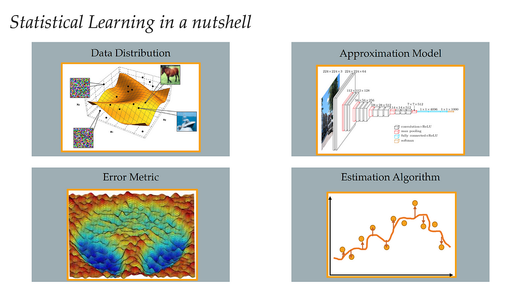
Statistical learning can be defined as the task of extracting information from possibly high-dimensional and noisy data, to give some guarantees of performance on unseen data. Since we want to do this task on a computer, basically we need four main ingredients:
- Data Distribution.
- Approximation Model: to process information (linear regression, SVM, NN, etc).
- Error Metric: to compare and choose between models.
- Estimation Algorithm: some procedure we can implement on the computer to find the estimate.
We’ll go through each ingredient in the next sections.
Data Distribution
In supervised learning, what will be focused on, consider the input data is a set of N samples, 𝒟= {(𝓍ᵢ, 𝓎ᵢ): i from 1 to N} drawn i.i.d. from an underlying data distribution 𝒫, defined over the input space 𝒳× the output space 𝒴. The feature 𝒳 in this definition is a high-dimensional space (𝒳=ℝᵈ). For simplicity, we will assume the output space is ℝ (the set of real numbers), and the labels 𝓎 comes from unknown function f* such that 𝓎ᵢ= f*(𝓍ᵢ) and hence f*: 𝒳→ ℝ.
For example, in the medical field, for diagnosing breast cancer, the input may be a histological image, with a categorical output that determines whether it is benign or malignant. This type of problem is called classification. For regression, perhaps in chemistry, we got a molecule, and we want to predict its excitation energy.
However, as we also know, we need some assumptions on the data for any kind of analysis in ML, because without assumptions on the distribution or the target we will not be able to generalize. These assumptions are essential for anything, and hence on geometric deep learning, as we will see later.
Approximation Model
The second ingredient in statistical learning is the model or the hypothesis class 𝓕, which is a subset of functions or mapping that goes from the input space 𝒳to the output space ℝ, 𝓕⊂ { f: 𝒳→ ℝ }.
Some examples of hypothesis classes could be:
- { Polynomials of degree up to k }
- { Neural networks of given architecture }
Let’s also define the complexity measure γ over the hypothesis class 𝓕, which will be like a norm or non-negative quantity we can evaluate in our hypothesis to divide it into simple and complicated, γ: 𝓕 → ℝ₊. Or in simple words, whether the set of allowed functions is too large or not.
The following can serve as examples for complexity measures:
- γ(f) could be the number of neurons in the neural network hypothesis.
- Or it could be the norm of the predictor.
We are interested in complexity measures because we want to control our hypothesis. Otherwise, we might get into a well-known problem called overfitting.
Error Metric
The error metric (also called the loss function) indicates the quality of the model output. Usually, we have different models, and we want to select the best one, for this reason, we use the error metric. It’s dependent on the task. In classification tasks, we use the accuracy, and in regression, we use the mean squared error. Mathematically, it is defined as a mapping 𝓁 from the tuple that contains the ground truth & the model output (𝓎, f(𝓍)) to the positive real numbers ℝ₊.
The loss function is a point-wise measure (we can measure the loss at every point in our data). So we need to consider the average for all our points. Obviously, have two fundamental notions of average in machine learning that are intricately connected; population average and empirical average. The population average (we call it also the excepted risk) is defined as the expectation for the data of the point-wise measure 𝓁(𝓎, f(𝓍)), i.e. how well we can do on average concerning the data distribution. Mathematically, given the loss function 𝓁, the model f, and the underlying data distribution 𝒫, defined over the input space 𝒳× the output space 𝒴, the expected risk 𝓡( f ) is defined as follows:︁︁︁

The second notion of average is the training loss or the empirical risk. We can drive this loss by replacing the expectation over the data in the above equation with the empirical expectation.

In fact, in all aspects of ML, what we are trying to do is to minimize the population error, but we don’t have access to this error, instead, we use the empirical one. You might ask how those two notions of average relate to each other. If you look at the empirical loss with a fixed f, i.e. if we fixed the hypothesis, it is the average of i.i.d, because every 𝓍ᵢ is a distributed i.i.d from the data distribution. Consequently, by some basic of elementary probability and statistics, and because the empirical loss is a random quantity that depends on the training set, the expectation of this loss will be the same as the expectation of the error metric, which is an unbiased estimator of the population loss.
Also, we can compute the variance point-wise, which is just by composing the random variable 𝓍ᵢ to the function f. Mathematically, for each f ∈ 𝓕, 𝓡( f̂ ) is an unbiased estimator of 𝓡(f), with variance 𝜎²(f) defined by:

However, this point-wise variance bound is not very useful in ML, since the relationship between the training and testing error we can not make it point-wise, because the hypothesis f depends on the training set. And so we need to do something instead which is called uniform bounds, e.g Rademacher complexity.
Estimation Algorithm
The last ingredient in statistical learning is the learning algorithm (or estimation algorithm). It’s defined as a function that goes from the dataset 𝒟= {(𝓍ᵢ, 𝓎ᵢ): i from 1 to N} to a function from the input space 𝒳 to the output space 𝒴. In simple terms, it’s an algorithm that’s output an algorithm!
We will discuss a popular prediction algorithm called empirical risk minimization (ERM). Hence our goal is to minimize a deterministic function (population loss or excepted risk) by only accessing a random function (training loss or empirical risk). As mentioned before, we have to control the distance between those two functions in a way that has to go beyond point-wise control.
Let’s define a ball with a radius 𝛿 in our hypothesis 𝓕, which has the complexity measure γ, such that:

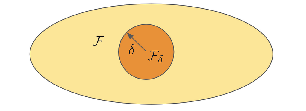
In other words, we have the space of all possible functions that we can implement using a neural network, for example, and we want to focus on those only with small complexity. Since we defined a set of smaller hypothesis in 𝓕 with radius 𝛿, we can consider an algorithm or estimator called empirical risk minimization (the function in the ball that happens to minimize the empirical risk), or in a constrained form:

Connecting to optimization, it may not be easy to use the constrained form in practice. So we need to consider another form, such as the penalized form and the interpolation form. In the penalized form, we introduce a Lagrange multiplier λ, where the constraint becomes part of the optimization objective (λ is a hyper-parameter that controls the strength of regularization).

The second form of the empirical risk minimization is the interpolation form, which is a very natural estimator, defined by the equation:

The empirical risk is zero means that the point-wise error is zero for every point in the data. Usually, we don’t want to do this in real life as the data contains noise.
Basic Decomposition of Error
After describing the four main actors in supervised learning, and since our goal is to minimize the population error, currently, we derive the various components of this population error.
Let f̂ be the model that’s we get from the learning algorithm (ERM). Then, 𝓡(f̂) will represent the population loss for this particular function. We will start by subtracting:

The term in brown is the infimum over all the hypothesis of the population; in other words, the best we could do in our hypothesis 𝓕. This term will be zero if 𝓕is dense, i.e. the ability to approximate almost arbitrary functions (Universal Approximation Theorem).
Then, we can write:

We call the green-colored term the Approximation Error (εₐₚₚᵣ), which indicates how well the functions of the smaller hypothesis can approximate the ground truth function. In other words, how well we can approximate the target function f* with small complexity.
Consequently, we reduce the above equation to:

Also, the term in red can be written as:

We call the blue term the Optimization Error (εₒₚₜ ), which compares the population objective with the training objective, and thus measures our ability to solve the empirical risk minimization (ERM) efficiently.
The other terms on the same side of the equation can be bounded by:

The last component in our decomposition (the orange-colored term) is the statistical error (εₛₜₐₜ ). This error penalizes uniform fluctuations over the ball (with radius δ) between the true function (the best function) and the random function (the training error).
Finally, the population error can be written as:

The Challenge of High-Dimensional Learning
Summarizing what we drive in the last section, we decomposed the population error into four components as follows:
1. Infimum over all the hypothesis of the population.
As mentioned before, this term will be zero if 𝓕 is dense, eg. neural networks with non-polynomial activation.

2. Approximation error.
The approximation error is a deterministic function that doesn’t depend on the size of the training data (number of samples). (Small if hypothesis space is such that target function has small complexity).

3. Statistical error.
This error is a random function that decreases when the number of samples increases. (Small when hypothesis space can be covered with ‘few’ small balls).

4. Optimization error.
Small when the ERM can be efficiently solved (in terms of iteration complexity).

Since we don’t have direct access to our population error, instead, we use the three different errors defined above as an upper bound for it (approximation, statistical, and optimization errors). When minimizing these errors, will guarantee to minimize our true objective (i.e. the population error). The pressing question here is how can we control these sources of error at the same time, when the data lives in high-dimensional space?
The Curse of Dimensionality
The curse of dimensionality was formulated by the American mathematician Richard Bellman in the context of dynamic programming and optimization, and it has since become almost synonymous with high-dimensional statistical learning. We are concerned about the curse of dimensionality because the basic principle of learning is fundamentally based on interpolation. For example, with the two classes of samples in the figure below, it is easy to agree on an architecture that interpolates each class from the given samples, which will be done by the learning algorithm.
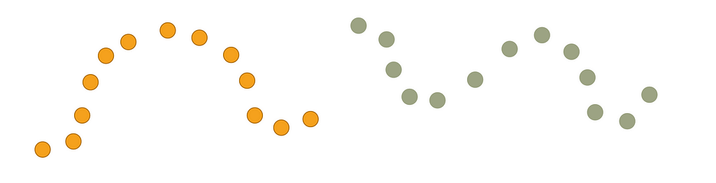
So the learning principle is based on a very basic property that we can extract the structure based on the proximity between empirical and population densities. The problem is that this learning principle suffers a lot in the higher dimensions. To convey the high-dimensional problems, let’s consider the following example.
Let’s first define the class of Lipschitz functions.
Lipschitz functions is a hypothesis of functions that is just like elementary fundamental regularity, only depends on locality. 1-Lipschitz functions f: 𝒳→ ℝ; the functions satisfying |f(𝓍) − f(𝓍´)| ≤ ||𝓍 − 𝓍´|| for all 𝓍, 𝓍´ ∈ 𝒳.
From this definition, assume the target function f* is 1-Lipschitz, and the data distribution 𝜈 is the standard Gaussian distribution. Then:
The number of samples N that are needed to estimate f* up to an error 𝜖 is: N = Θ (𝜖⁻ᵈ), where d is the number of dimensions. (For the proof, GDL proto-book, section 2.2).
It is evident that the number of samples grows exponentially in dimension, indicating that the Lipschitz class grows too fast as the input dimension increases. This situation will not be better if we replace the Lipschitz class with a global smoothness hypothesis, such as the Sobolev class, as we will see in the next section.
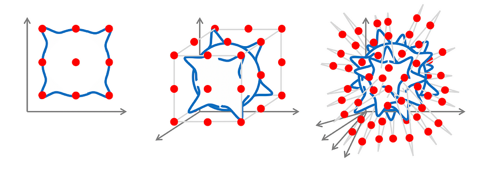
Curse in Approximation
After explaining the curse of dimensionality, we want to show that this curse appears in many other contexts. For example, it can also come out in just a pure approximation.
Let’s consider a neural network model that has only one hidden layer, the class of functions that we can write as a linear combination of simple activation functions. This hypothesis class has a very natural notion of complexity, which is the number of neurons in the hidden layer.
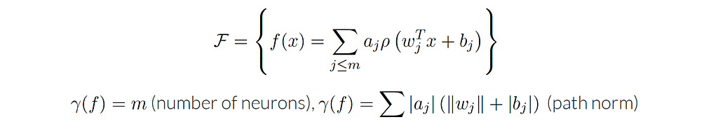
With Universal Approximation Theorem, we can approximate almost arbitrary functions using this hypothesis class. And here, the essential question will be what is the approximation rate? As mentioned before, we are interested in approximation errors that work at finite δ. We want to control the complexity, for this reason, we want to look at the difference between the approximation over the entire hypothesis space and the approximation over a subset of the hypothesis space that has a small complexity. Therefore, how do we approximate functions with a small number of neurons?
Unfortunately, these rates of approximation are also cursed. If we take, for example, a simple class of functions, Sobolev class, f∈ ℋˢ (s: number of finite derivatives of f). Then:

Curse in Optimization
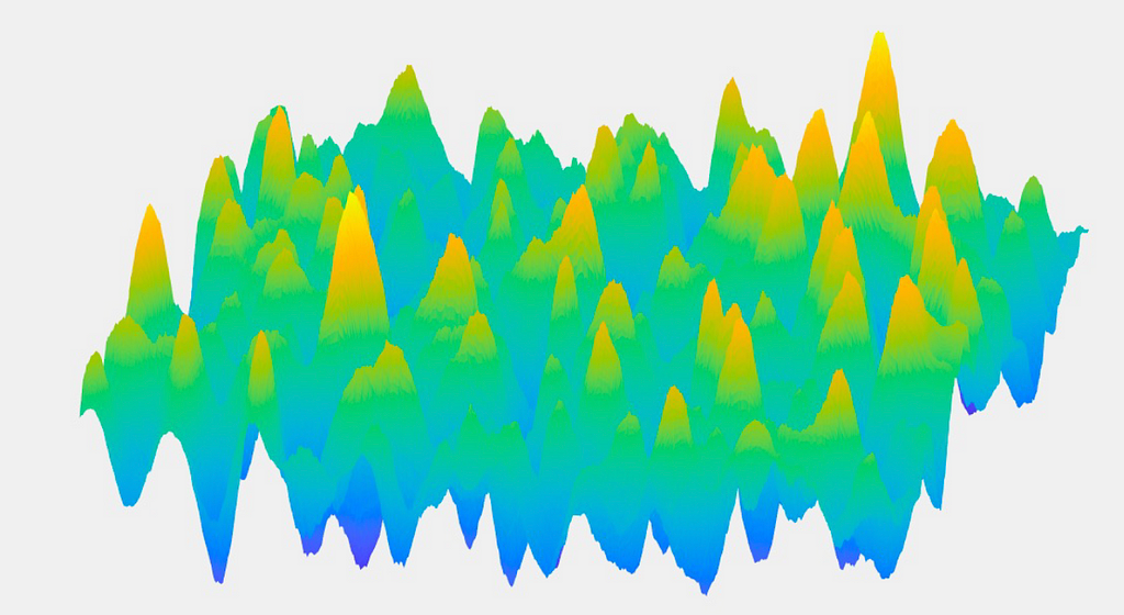
Another curse also appears in high-dimensional learning, the curse of dimensionality in optimization. Suppose we want to find the global minima for the landscape defined in the image below. A priori, we need to visit every possible point and store the minimum location. In other words, we have to go over all the space and evaluate every possible point to determine the minimum one. This process has an exponential dependency in dimensions (NP-hard). And so it’s the same story again, there’s an exponential blow-up of complexity. Consequently, how do we usually overcome this curse in practice?
In many ML problems, the scene is simpler than the one defined above. It is like the one in the picture below (there is always a decent path). In more mathematical terms, many of the landscapes we care about don’t have many bad local minima; the places where we will stick in the landscape are not very large. It is not like the worst case where we have an exponential number. This sense simplifies the problem if we can have a practical understanding of how expensive it is to find a local minima for a function instead of finding a global minima that we know in the worst case is exponential.

Practically, it is easy to find a local minima in high dimensions, since the gradient descent can find a local minima efficiently (in terms of iteration complexity); no exponential dependency in dimension.
Theorem [Jin et al.´17]: Noisy Gradient Descent finds ε-approximate second-order stationary points of a β-smooth function in Õ(β/ε²) iterations.
However, this situation is not always true, there are still many problems in ML where assuming “there is no bad local minima” is not true.
Summary so far
Up to now, we’ve discussed the curse of dimensionally and how it appears in the statistical error when assuming a pretty large class such as Lipschitz functions. In contrast, if we tried to impose stronger assumptions about regularity to make the problem easier, considering the Sobolev class, for example, the approximation error will be cursed by dimension.
Thus we need to break this paradigm. Accordingly, the question would be, how do we define more adapted function spaces?
Towards Geometric Function Spaces
In fact, each point in our data is not just a point in a high-dimensional space. It can also be considered as a signal, where each point in itself is a function. The high dimensional space 𝒳 is hiding inside a low dimensional structure, and this low dimensional structure can be a grid in 2d, group, sphere, graph, mesh, etc. We will discuss this in detail in later posts.
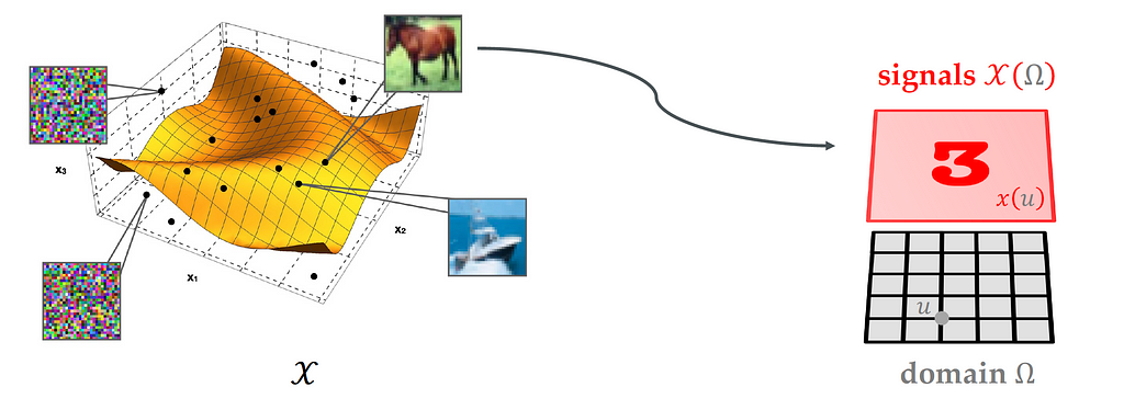
The main question here is can we exploit this geometric domain to find a new notion of regularity that we use to overcome these limitations that we have just discussed in classical spaces functions?
The answer to this question is one of the main objectives of geometric deep learning (GDL), as you will see in our subsequent posts.
In this post, we have discussed the statistical learning task, and the main three errors that we should be concerned about. We showed that high-dimensional learning is impossible without assumptions due to the curse of dimensionality, and that the Lipschitz & Sobolev classes are not good options. Finally, we introduced the geometric function spaces, since our points in high-dimensional space are also signals over low-dimensional geometric domains. In the next post, we will see how these geometric structures can be used to define a new hypothesis space using invariance and symmetry, as defined by geometric priors.
References:
- GDL Course, (AMMI, Summer 2021).
- Lecture 2 by J. Bruna [ Video | Slides ].
- M. M. Bronstein, J. Bruna, T. Cohen, and P. Veličković, Geometric Deep Learning: Grids, Groups, Graphs, Geodesics, and Gauges (2021).
- F. Bach, Learning Theory from First Principles (2021).
We thank Rami Ahmed for his helpful comments on the draft.
High-Dimensional Learning was originally published in Towards Data Science on Medium, where people are continuing the conversation by highlighting and responding to this story.
from Towards Data Science - Medium https://ift.tt/npGMJXF
via RiYo Analytics


No comments