https://ift.tt/31HTqYQ Learn the details behind this everyday tool from the Topic Modeling toolbox Photo by Isaac Smith on Unsplash I...
Learn the details behind this everyday tool from the Topic Modeling toolbox

If you are familiar with Topic Modeling, you probably already heard about Topic Coherence or Topic Coherence Metrics. In most articles about Topic Modeling, it is shown as a number that represents the overall topics’ interpretability and is used to assess the topics’ quality.
But, what exactly is this metric? How it’s capable of measuring the ‘interpretability’? We should look to maximize it at all costs?
In this post, we gonna dive into this topic to answer these questions and give you a better understanding of Topic Coherence Measures.
Let’s open this black box.
Summary
I. Remembering Topic Model
II. Evaluating Topics
III. How Topic Coherence Works
- Segmentation
- Probability Calculation
- Confirmation Measure
- Aggregation
- Putting everything together
IV. Comprehending models in Gensim
V. Applying in some examples
VI. Conclusion
References
I. Remembering Topic Model
Topic Modeling is one of the most important NLP fields. It aims to explain a textual dataset by decomposing it into two distributions: topics and words.
It is based on the assumption that:
- A text (document) is composed of several topics
- A topic is composed of a collection of words
So, a Topic Modeling Algorithm is a mathematical/statistical model used to infer what are the topics that better represent the data.
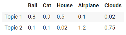
For simplicity, a topic can be described as a collection of words, like [‘ball’, ‘cat’, ‘house’] and [‘airplane’, ‘clouds’], but in practice, what an algorithm does is assign each word in our vocabulary a ‘participation’ value in a given topic. The words with the highest values can be considered as the true participants of a topic.
Following this logic, our previous example will be something like this:
II. Evaluating Topics
Computers are not humans. As described before, topic modeling algorithms rely on mathematics and statistics. However, mathematically optimal topics are not necessarily ‘good’ from a human point of view.
For example, a topic modeling algorithm can find the following topics:
- Topic 1: Cat, dog, home, toy. (Probably a good topic)
- Topic 2: Super, nurse, brick. (Probably a bad topic)
From a human point of view, the first topic sounds more coherent than the second but, for the algorithm, they are probably equally correct.
Sometimes, we don't need that the topics created to follow some interpretable logic, and we just want to, for example, reduce the data dimensionality to another machine learning process.
When we’re looking for data understanding, the topics created are meant to be human-friendly. So, just blindly following the inherent math behind topic model algorithms can lead us to misleading and meaningless topics.
Because of this, topics’ assessment was usually complemented by qualitative human evaluations, such as reading the most important words in each topic and seeing the topics related to each document. Unfortunately, this task can be very time-consuming and impracticable to very large datasets with thousands of topics. It also requires prior knowledge about the dataset’s field and may require specialist opinions.
This is the problem Topic Coherence Measures try to solve. They try to represent the ‘quality human perception’ about topics in a unique, objective, and easy-to-evaluate number.
III. How Topic Coherence Works
The first key point to understand how these metrics work is to focus on the word ‘Coherence’.
Usually, when we talk about coherence, we talk about a cooperation characteristic. For example, a set of arguments is coherent if they confirm each other.
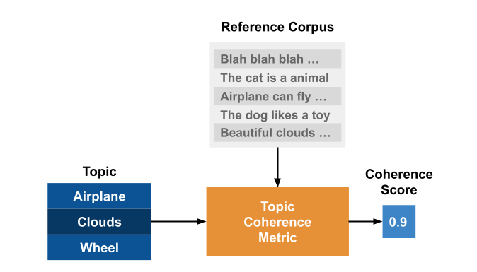
What a Topic Coherence Metric assesses is how well a topic is ‘supported’ by a text set (called reference corpus). It uses statistics and probabilities drawn from the reference corpus, especially focused on the word’s context, to give a coherence score to a topic.
This fact highlights an important point of the topic coherence measures: it depends not only on the topic itself but also on the dataset used as reference.
Röder, M. et al in Exploring the Space of Topic Coherence Measures proposes a general structure a topic coherence metric follows:
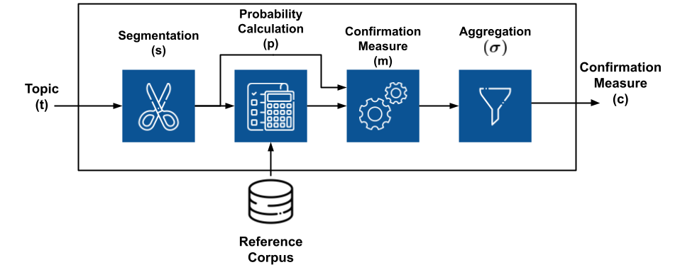
It's a composition of different independent modules, each one doing a specific function, that is joined together in a sequential pipeline.
That is, the topic coherence measure is a pipeline that receives the topics and the reference corpus as inputs and outputs a single real value meaning the ‘overall topic coherence’. The hope is that this process can assess topics in the same way that humans do.
So, let's understand each one of its modules.
Segmentation
The segmentation module is responsible for creating pairs of word subsets that we’re gonna use to assess the topic’s coherence.
Considering W={w_1, w_2, …, w_n} as the top-n most important words of a topic t, the application of a segmentation S results in a set of subset pairs from W.

Where the second part of the pair (W*) is gonna be used to confirm the first part (W’). This will become clearer when we talk about probability calculation and confirmation measures in the next sections, where these pairs are gonna be used.
To simplify things, we can understand the segmentation as the step where we choose how we gonna ‘mix’ the words from our topic to evaluate them posteriorly.
For example, the segmentation S-one-one, says that we need to make word pairs of different words. So, if W = {‘cat’, ‘dog’, ‘toy’}, we gonna have:

So, by using this technique, we’re saying that to compute the final coherence score, our model is interested in the relationship between any two words of our topic.
Another example is the segmentation S-one-all, which says that we need to make pairs of each word with all other words. Applying it to W, we found:

Again, by using this technique, we’re saying that our coherence score will be based on the relation between a single word and the rest of the words in our topic.
Probability Calculation
As mentioned before, coherence metrics use probabilities drawn from the textual corpus. The Probability Calculation step defines how these probabilities are calculated.
For example, let's say we’re interested in two different probabilities:
- P(w): The occurrence probability of word w
- P(w1 and w2): The occurrence probability of words w1 and w2
Different techniques will estimate these probabilities differently.
For example, the Pbd (bd stands for boolean document) calculate P(w) as the number of documents that word w occurs divided by the total number of documents and P(w1 and w2) as the number of documents that both words occurs divided by the total.
Another example is Pbs (bs stands for boolean sentence), which does the same as the previous method but it considers the occurrences in the sentences, not in the full documents. Another example is Psw (sw stands for sliding window), which considers the occurrences in a sliding window over the texts.
These probabilities are the fundamental bricks of coherence. They are used in the next step to consolidate the score of the topic.
Confirmation Measure
The confirmation measure is the core of the topic coherence.
The confirmation measure is calculated over the pairs S using the probabilities calculated in P. It computes ‘how well’ the subset W* supports the subset W’ in each pair.
That is, this step tries to quantify the ‘relation’ between these two subsets by using the probabilities calculated from the corpus. So, if the words of W’ are connected with the words in W* (by, for example, being very often in the same document), the confirmation measure will be high.
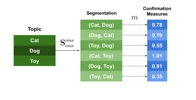
In the image above, we can see an example of this process. The confirmation measure m is applied to each one of the pairs created in the segmentation step, outputting the confirmation score.
There are two different types of confirmation measures, that we’re gonna understand in the following lines.
Direct confirmation measures
These measures compute the confirmation value by directly using the subsets W’ and W* and the probabilities. There is a world of direct measures that you can explore, but let’s stay with just a few examples:


We’re not going to dive into the math behind these equations, but keep in mind that they are derived from many scientific fields, such as Information Theory and Statistics.
Indirect confirmation measures
In summary, indirect confirmation measures do not compute a score based on W’ and W* directly. Instead, they compute a direct confirmation measure m over the words in W’ with all other words in W, building a measure vector, as shown below:

The same process is done to W*.
The final confirmation measure is the similarity (for example, cosine similarity) between these two vectors.

The image below shows an example of how this process is done. To compute the confirmation measure in the pair (‘cat’, ‘dog’), we first compute the confirmation measure m of each one of the elements with all the words in the topic, creating a confirmation measure vector. Then, the final confirmation measure is the similarity between these two vectors.
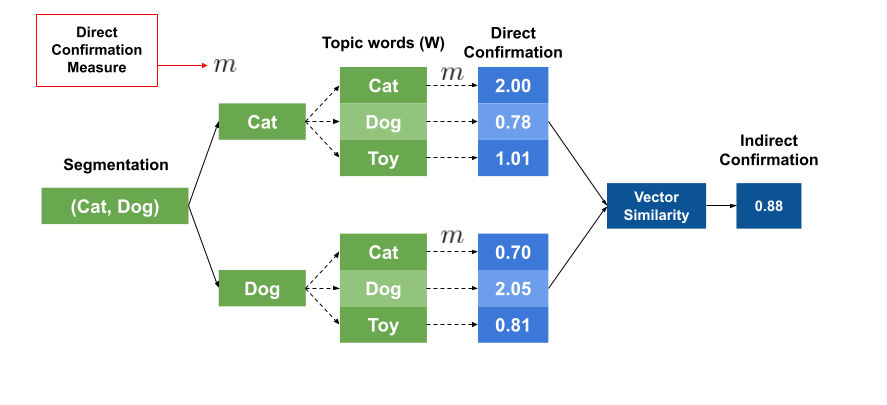
The idea behind this process is to highlight some relations that the direct method can miss. For example, the words ‘cats’ and ‘dogs’ may never appear together in our dataset, but they might appear frequently with the words ‘toys’, ‘pets’, and ‘cute’. With the direct method, these two words will have a low confirmation score, but with the indirect method, the similarity may be highlighted, since they occur in similar contexts.
With these measures calculated, we can move to the next step.
Aggregation
This is the last and simplest step.
It takes all the values calculated in the previous step and aggregates them into a single value, which is our final topic coherence score.
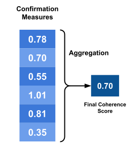
This aggregation could be the arithmetic mean, the median, the geometric mean, and so on.
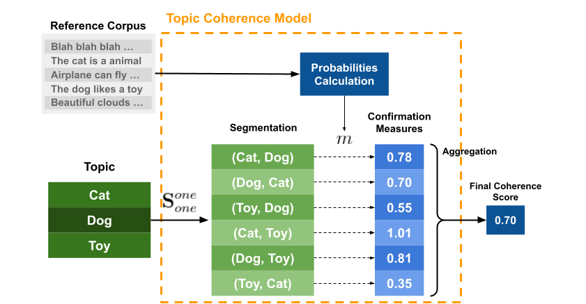
Putting everything together
So let’s review the steps.
- We had a topic that we want to evaluate.
- We choose a reference corpus.
- The top-n most important words in the topic were found, we called they W.
- W was segmented into pairs of subsets using a technique s.
- Using the reference corpus, we calculated word probabilities with a technique p.
- With the segmented words and the probabilities, we use a confirmation measure m to evaluate the ‘relation’ between the subsets of each pair.
- All the measures from the previous step are aggreged in a single final number, that is our Topic Coherence Score.
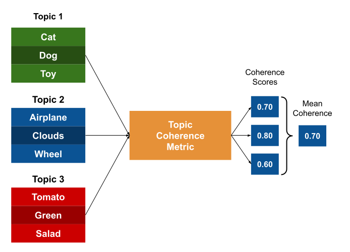
All these steps can be summarized in the image below:
In the case where we have many topics (which is the most usual), the final result is just the mean individual Topic Coherence.
IV. Comprehending models in Gensim
Ok, now that we learned how a Topic Coherence Measure works, let's apply our knowledge in a real example.
The Gensim library provides a class that implements the four most famous coherence models: u_mass, c_v, c_uci, c_npmi. So, let’s break them into fundamental pieces.
If we look at the paper (Röder et al, 2015), we gonna find that the authors already detailed how these coherence models are built.
So, to understand a model, we just need to understand its components.
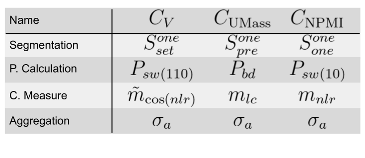
Let's take C_NPMI for example.
- Segmentation: It uses the method S-one-one, that is, the confirmation measure will be computed over pairs of words.
- Probability Calculation: It uses the method Psw(10). The probabilities are calculated over a sliding window of size 10 that moves over the texts.
- Confirmation Measure: The confirmation measure of each pair will be the Normalized Pointwise Mutual Information (NPMI).

- Aggregation: The final coherence is the arithmetic mean of the confirmation measures.
Let's also analyze the method C_V.
- Segmentation: It uses the method S-one-set, that is, the confirmation measure will be computed over pairs of a word and the set W.
- Probability Calculation: It uses the method Psw(110). The probabilities are calculated over a sliding window of size 110 that moves over the texts.
- Confirmation Measure: It uses an indirect confirmation measure. The words of each pair’s elements are compared against all other words of W using the measure m_nlr. The final score is the cosine similarity between the two measures vectors.
- Aggregation: The final coherence is the arithmetic mean of the confirmation measures.
To better understand the notations, I strongly recommend checking the original paper.
V. Applying in some examples
For our luck, we don’t need to know all these details to use the metrics with Gensim.
So, as a final exercise, let's evaluate some topics using the dataset 20newsgroups as our reference corpus.
First of all, let's import the libraries needed.
Then, let's fetch and tokenize the texts.
Using the coherence model in Gensim is very simple, we just need to create a set of topics and pass our texts. The code below creates some topics that we want to evaluate.
I chose specific topics that I already know work in this database.
The method .get_coherence_per_topic() return the coherence value for each topic. Let’s visualize the results using Seaborn.
The result is shown below.
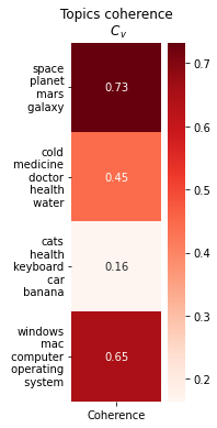
VI. Conclusion
Topic Modeling is one of the most relevant topics in Natural Language Processing, serving as a powerful tool for both supervised and non-supervised machine learning applications.
Topic Coherence is a very important quality measure for our topics. In this post, we dived into the fundamental structure and math behind the Topic Coherence Measures. We explored the blocks that compose a Topic Coherence Measure: Segmentation, Probability Calculation, Confirmation Measure, and Aggregation, understanding their roles. We also learned about the main topic coherence measures implemented in Gensim, with some code examples.
I hope that you find yourself more confident in working with these measures. The world of topic coherence is huge, and I strongly recommend further reading about it.
Thank you for reading.
References
[1] Röder, M., Both, A., & Hinneburg, A. (2015). Exploring the space of topic coherence measures. In Proceedings of the eighth ACM international conference on Web search and data mining (pp. 399–408).
[2] Rehurek, R., & Sojka, P. (2011). Gensim–python framework for vector space modeling. NLP Centre, Faculty of Informatics, Masaryk University, Brno, Czech Republic, 3(2).
Understanding Topic Coherence Measures was originally published in Towards Data Science on Medium, where people are continuing the conversation by highlighting and responding to this story.
from Towards Data Science - Medium https://ift.tt/3r6nENL
via RiYo Analytics


ليست هناك تعليقات