The Power of SQL Aggregate Window Functions with Disney Data

https://ift.tt/3KAQ6jN AVG(), COUNT(), MAX(), MIN(), SUM() Photo by Travis Gergen on Unsplash Window functions allow us to conduct oper...

https://ift.tt/3KAQ6jN

AVG(), COUNT(), MAX(), MIN(), SUM()

Photo by Travis Gergen on Unsplash

Window functions allow us to conduct operations and display the results on each row, as opposed to normal SQL operations that combine multiple rows based on your query. Normal SQL aggregate functions are essential for breaking down multiple rows into solutions. These functions for example, may show the average of multiple rows and output a single numeric value, or show the count of instances within a group of rows. In aggregate window functions, we can apply this aggregate result to every row of the data. This allows us to easily create useful, and efficient, results such as cumulative sum, comparisons of specific rows output vs averages over all rows.

The five types of aggregate window functions are:

• AVG()
• COUNT()
• MAX()
• MIN()
• SUM()

Before we get into the details of each aggregate window function, we should look into how these functions are generally written out:

[Aggregate Function]([column]) OVER([specific operation] column_name)

For example, a sample SQL command would look like:

SELECT *, SUM(column_x) OVER(PARTITION BY column_y ORDER BY column_z)
FROM table

*Note that the columns x, y, & z may be the same or different*

Data:
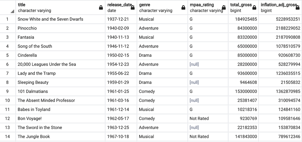
The data used in this article was originally posted to Kaggle by Rashik Rahman and is licensed as CC0: Public Domain. The link to Rashik’s Kaggle profile can be found (here). The data is comprised of Disney movies from the years 1937–2016 and shows the following variable names: movie title, movie release date, genre, mpaa rating, total gross, and inflation adjusted gross. For the purposes of this article, I will mostly be using ‘title’, ‘release_date’, ‘genre’ and ‘total_gross’. Additionally, I will focus on movies released in the year 2015 to simplify the resulting outputs. A sample of the data is below:

Image by Author

*This data will only be used for demonstrating our aggregate window functions, and should not be regarded as a complete and accurate source for these films.

Basic Use Cases:
As mentioned earlier, aggregate window functions work the same way as normal aggregate functions but rather than providing a consolidated output, the output is reflected on each row in the table. For example, the AVG() window function does exactly what you’d expect, it creates an average of the values in the given partition and outputs this value onto each row of the data. The SQL code below demonstrates just that:

SELECT title, genre, total_gross, 
ROUND(AVG(total_gross) OVER(PARTITION BY genre),0) as average 
FROM disney
WHERE release_date >= '2015-01-01' AND release_date < '2016-01-01'

Image by Author

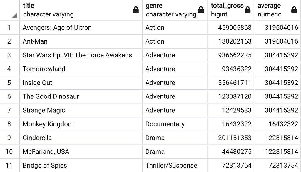
The new column ‘average’, partitioned by genre, displays the average of each genre’s gross box office earnings. Using the same concept and practice, we can run similar metrics using all five of the aggregated functions.

SELECT title, genre, total_gross, 
ROUND(AVG(total_gross) OVER(PARTITION BY genre),0) as average,
ROUND(COUNT(*) OVER(PARTITION BY genre),0) as total_count,
ROUND(MAX(total_gross) OVER(PARTITION BY genre),0) as max_gross,
ROUND(MIN(total_gross) OVER(PARTITION BY genre),0) as min_gross,
ROUND(SUM(total_gross) OVER(PARTITION BY genre),0) as total_sum
FROM disney
WHERE release_date >= '2015-01-01' AND release_date < '2016-01-01'

Image by Author

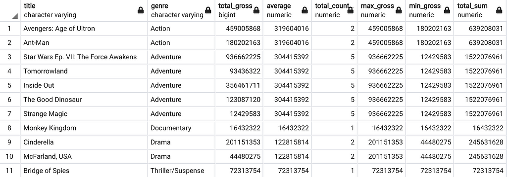
Here we see each of the aggregate functions used and each of their outputs. While obtaining this information can be helpful, this type of operation could also be done without the window function and instead with a normal aggregate nested query joined to our original dataset. An example of this is shown below with the AVG() function:

SELECT title, d.genre, total_gross, ROUND(average,0)
FROM disney d LEFT JOIN 

(SELECT genre, AVG(total_gross) as average 
 FROM disney
 WHERE release_date >= '2015-01-01' AND release_date < '2016-01-01'
 GROUP BY genre) a

ON d.genre = a.genre

WHERE release_date >= '2015-01-01' AND release_date < '2016-01-01'
ORDER BY genre

The result of the above code block is the exact same as our window function, however the above code block requires a more complicated statement.

Cumulative Cases:
In my opinion, the greatest advantage of these aggregate window functions is when they are used to find cumulative values. To make this change to our existing code block all we need to do is add the ORDER BY clause in our OVER() statement. Being able to add cumulative values in a few steps helps to add tremendous strength to these aggregate window functions. An example of this principle is shown below using the SUM() function.

SELECT title, genre, total_gross, 
ROUND(SUM(total_gross) OVER(PARTITION BY genre ORDER BY release_date),0) as cumulative_sum
FROM disney
WHERE release_date >= '2015-01-01' AND release_date < '2016-01-01'

Image by Author

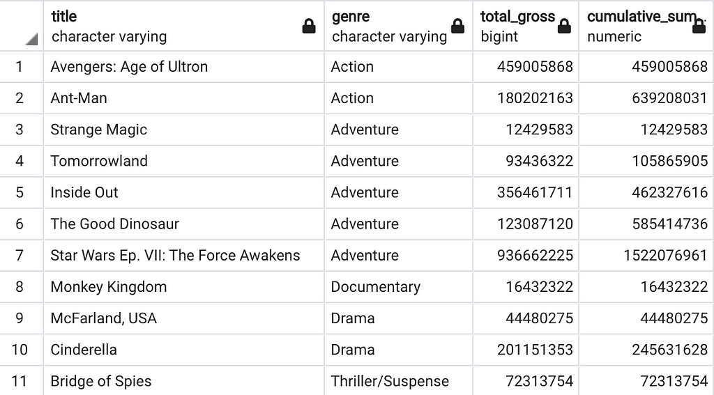
Here we see the cumulative aspects of the total_gross column for each partition. We can apply this same method to all the functions using the code block below:

SELECT title, genre, total_gross, 

ROUND(AVG(total_gross) OVER(PARTITION BY genre ORDER BY release_date),0) as cumulative_average,

ROUND(COUNT(*) OVER(PARTITION BY genre ORDER BY release_date),0) as cumulative_count,

ROUND(MAX(total_gross) OVER(PARTITION BY genre ORDER BY release_date),0) as max_gross,

ROUND(MIN(total_gross) OVER(PARTITION BY genre ORDER BY release_date),0) as min_gross,

ROUND(SUM(total_gross) OVER(PARTITION BY genre ORDER BY release_date),0) as cumulative_sum

FROM disney
WHERE release_date >= '2015-01-01' AND release_date < '2016-01-01'

Image by Author

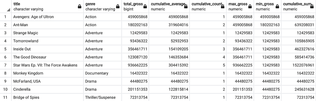
Using the cumulative features of these functions, we can now see some interesting results. Looking at the ‘Action’ genre as an example, we can see the average started out as $459M following the first film ‘Avengers: Age of Ultron’ before falling to an average of $320M following the inclusion of ‘Ant-Man’. The cumulative_count column simply counts the number of rows and displays the result. We see the max_gross column remains at $459M for both films because the first film was higher grossing than the second, conversely, when looking at min_gross we see that it starts at $459M before falling to $180M after ‘Ant-man’ is observed. Lastly, the cumulative_sum works as we had explained prior, by adding each film’s total_gross within the partition.

Conclusion:
Using aggregate window functions can help us create useful and informative metrics, while also helping us save time while writing queries. Aggregate window functions are just one branch of window functions, you can find my prior article about ranking window functions here. Thank you for taking the time to read this article, please follow me for more data science related content!

Image by Author

---

The Power of SQL Aggregate Window Functions with Disney Data was originally published in Towards Data Science on Medium, where people are continuing the conversation by highlighting and responding to this story.

from Towards Data Science - Medium https://ift.tt/3KJbPX9
via RiYo Analytics