https://ift.tt/39zmguG A hands-on tutorial which demonstrates how to utilize the Pandas package to clean, manipulate, and analyze data. I...
A hands-on tutorial which demonstrates how to utilize the Pandas package to clean, manipulate, and analyze data.

1. Introduction
Have you ever struggled to analyze big datasets in Excel then, you should have considered Pandas, powerful programming and data analysis toolbox which allows you to manipulate million-row data points in milliseconds with high processing power and user productivity. In fact, Pandas is an open-source python library, introduced by software developer Wes McKinney in 2008, which includes high-level data structures and programming tools to perform data analysis and manipulation on different data types whether numbers, text or dates, etc. This tutorial provides the necessary knowledge for you to start applying Pandas in your projects.
2. Objective
Let us consider you just joined a startup as a data analyst and you have been assigned to support the team to drive insights about the customers base. Your manager shared the dataset and here is your opportunity to showcase your python skills and use the Pandas package to perform the analysis.
This tutorial will help you to develop and use Pandas knowledge to:
1- import and read a CSV file
2- generate a basic understanding of a given data
3- select and filter data based on conditions
4- apply various data operation tools such as creating new variables or changing data types
5- perform data aggregation using group by and pivot table methods
6- transform analytical insights into business recommendations.
#laod the needed packages and modules
import pandas as pd
import numpy as np
from datetime import date
import datetime as dt
3. Data Analysis
3.1 Load the data
The first step is to load the data using pd_read_csv which reads the data of a CSV file, loads and returns the content in a data frame. You might ask yourself, what is a data frame? Data frames are the primary data structure in the pandas package which displays the data in a table of different attributes as shown below. For more information about the pd.read_csv, visit the link.
The dataset which will be used in this tutorial is a dummy dataset was created for this article. It is available in this link and it includes interesting data about customers which can be used in a targeted marketing campaign.
#load the data and make sure to change the path for your local
directory
data = pd.read_csv('C:/Users/Smart PC/Desktop/project_data.csv')
3.2 Gain basic understanding
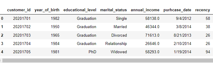
After we loaded the data, we can use different methods to view and understand the variables. For example, data.head() enables us to view the first 5 rows of the dataframe whereas data.tail() returns the last 5 rows. If you want to get the first 10 rows, you need to specify it in the method as data.head(10).
#first 5 rows
data.head()
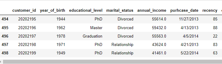
#last 5 rows
data.tail()
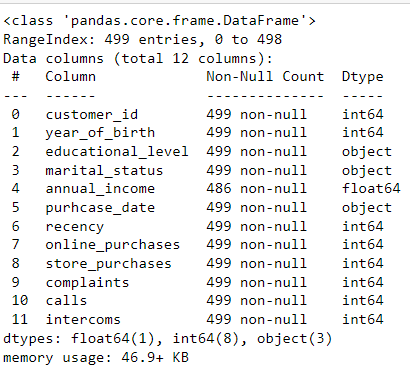
Another interesting method is data.info() which gives us the number of data points and variables of the dataset. It also displays the data types. We can see that our dataset has 499 data points and 12 variables ranging from customers’ personal information to purchases, calls, intercoms, and complaints.
#check the basic information of the data
data.info()
We can check the shape of the dataset using data.shape; it indicates that our dataset has 449 rows and 12 columns.
#extract the shape of the data
data.shape
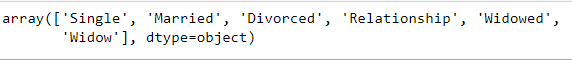
Let us consider we are interested to know the unique values of the marital status field then, we should select the column and apply the unique method. As shown below the variable marital status has 5 unique categories. However, we notice that widow and widowed are two two different naming for the same category so we can make it consistent through using replace method on the column values as displayed below.
data['marital_status'].unique()
data[‘marital_status’] = data[‘marital_status’].replace(‘Widow’, ‘Widowed’)
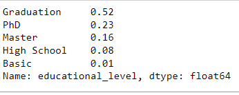
Another interesting way to know the unique values but with their respective counts is to apply the value_count method on the column. For instance, the education attribute has 5 categories whereby Graduation and PhD constitute the largest proportion.
round(data['educational_level'].value_counts(normalize=True),2)
We can check for duplicates and null values in the whole dataset using the .duplicated and .isnull methods. Furthermore, we can select one variable of interest in the dataset to detect its missing values or duplicates as displayed below.
data.isnull()
data.duplicated().sum()
data['educational_level'].isnull().sum() #specifying Education as a variable where we should look for the sum of missing values
3.3 Select and filter data: loc and iloc
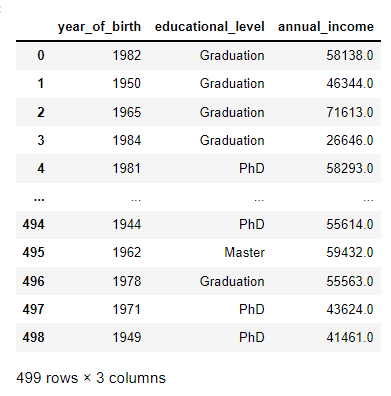
We can simply select a subset of the data points from the data frame. Let us consider that we want to select the Birthdate, Education, and Income of every customer; this is achievable through selecting the column names with double brackets as shown below.
subset_data = data[['year_of_birth ', 'educational_level', 'annual_income']]
subset_data
We can select a unique category of the education by specifying that only “Master” should be returned from the data frame.
data[data["educational_level"] == "Master"]

The other two popular methods to select data from a data frame are: loc and iloc. The main distinction between these two methods is that: loc is label-based, which means that we have to specify rows and columns based on the titles. However, iloc is integer position-based, so we have to select the rows and columns by their position values as integer i.e: 0,1,2. To read more about selecting data using these methods, visit this link.
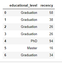
As we notice below, we are selecting the first seven data points using the loc method, but for the variables ‘educational_level’ and ‘recency’. We can also achieve the same result with iloc but with specifying the rows and columns as integer values.
data.loc[:6, ['educational_level', 'recency']] #specify the rows and columns as labels
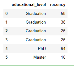
data.iloc[:6, [2,6]] #speciy rows and columns as integer based values
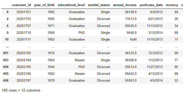
Another powerful tool is to filter data using the loc and isin() methods whereby we choose the variable of interest and we select the categories we want. For example, below we are choosing all the customers with a Marital Status described as Single or Divorced only.
data.loc[data[‘marital_status’].isin([‘Single’, ‘Divorced’])]
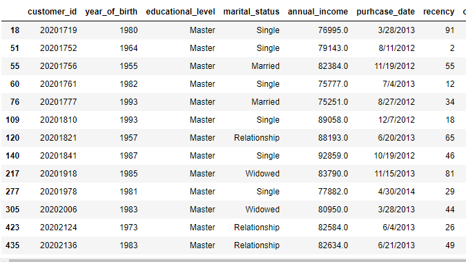
We can combine iloc with a python operator to select data that satisfies two conditions such as choosing the customers with an income higher than 75,000 and with a master’s degree.
data.iloc[list((data.annual_income > 75000) & (data.educational_level == 'Master')), :,]
3.4 Apply data operations: index, new variables, data types and more!
We can apply different operations on the dataset using Pandas such as but not limited to:
- setting a new index with the variable of our interest using the .set_index() method
- sorting the data frame by one of the variable using .sort_values() with ascending or descending order; For more information about the sort_values(), visit the link
- creating a new variable which could be the result of a mathematical operation such as sum of other variables
- building categories of a variable using pd.cut() method; For more information about the pd.cut(), visit the link
- changing the datatype of variables into datetime or integer types
- determining the age based on year of birth
- creating the week date (calendar week and year) from the purchase date
and many more; this is just a glimpse of what we can achieve with pandas!
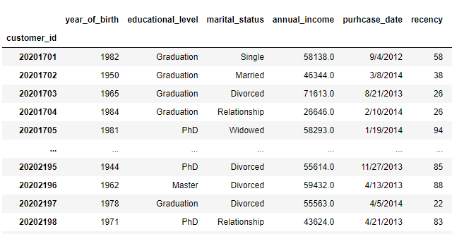
#set the index as customer_id
data.set_index(‘customer_id’)
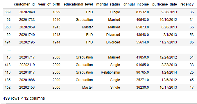
#sort the data by year_of_birth, ascending is default;
data.sort_values(by = ['year_of_birth '], ascending = True) # if we want it in descending we should set ascending = False
#create a new variable which is the sum of all purchases performed by customers
data['sum_purchases'] = data.online_purchases + data.store_purchases
data['sum_purchases']

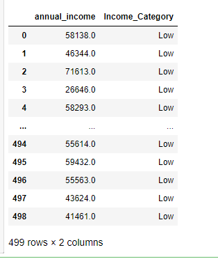
#create an income category (low, meduim, high) based on the income variable
income_categories = ['Low', 'Meduim', 'High'] #set the categories
bins = [0,75000,120000,600000] #set the income boundaries
cats= pd.cut(data['annual_income'],bins, labels=income_categories) #apply the pd.cut method
data['Income_Category'] = cats #assign the categories based on income
data[['annual_income', 'Income_Category']]
#we can change the datatype of purchase_date to datetime and year_birth to integer
data['purhcase_date'] = pd.to_datetime(data['purhcase_date'])
data['year_of_birth '] = data['year_of_birth '].astype(int)
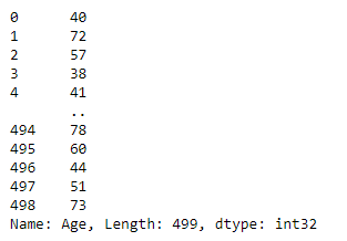
#find out the age of customers based on the current year
today = date.today()
year = int(today.year)
data['Age'] = year - data['year_of_birth ']
data['Age']
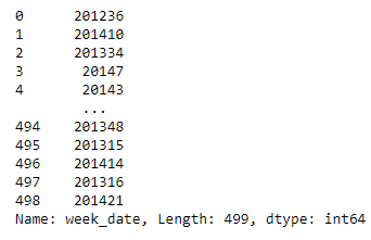
#extract the week_date from the purchase_date which shows the year of purchase and the calendar week
#make sure to change the purhcase_date varibale to datetime as shown above before applying the .isocalendar() method
data["week_date"] = [int(f'{i.isocalendar()[0]}{i.isocalendar()[1]}') for i in data.purhcase_date]
data["week_date
3.5 Perform data aggregation: groupby and pivot_table
After we created new variables, we can further aggregate to generate interesting insights from categories. Two key methods every data scientist uses to analyze data by groups:
- groupby(): a method that involves splitting categories, applying a function, and combining the results, whereby it can be used with a mathematical operation such as mean, sum, or count with an aggregated view by a group. For further information about this operation, visit this link
2. pivot_table() : a very useful technique that creates a spreadsheet-style pivot table as a Data frame, and it also allows analysts to apply a mathematical operation on selected variables per group. For further information about this pivot_table, visit this link
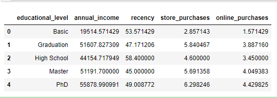
#apply groupby to find the mean of income, recency, number of web and store purchases by educational group
aggregate_view = pd.DataFrame(data.groupby(by='educational_level')[['annual_income', 'recency', 'store_purchases',  'online_purchases']].mean()).reset_index()
aggregate_view
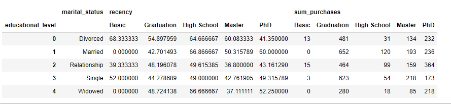
#apply pivot table to find the aggregated sum of purchases and mean of recency per education and marital status group
pivot_table = pd.DataFrame(pd.pivot_table(data, values=['sum_purchases', 'recency'], index=['marital_status'],
                        columns=['educational_level'], aggfunc={'recency': np.mean, 'sum_purchases': np.sum}, fill_value=0)).reset_index()
pivot_table
4. Recommendations
Now after we completed the process of data cleaning and performing operations and aggregations on our dataset, we can conclude with some interesting insights about our customer base:
- PhD people have the highest income, number of online and store purchases; however, High School graduates people have the highest recency or number of days since their last purchase
- Basic people account for the lowest number of web and store purchases
- Married people with Graduation level have the highest total purchases
Therefore, the business recommendations for any potential marketing campaign should focus on attracting and retaining PhD people and married couples with Graduation level, and more products should be offered to satisfy the needs and interests of other categories such as Basic people that have the lowest purchases as well as High School people who are not purchasing regularly.
Additionally, further work should be conducted to understand customer behaviors and interests, for example, performing RFM analysis or regression modeling will be beneficial to study the effect of variables on the number of purchases by educational or marital status group.
5. Conclusion
Finally, I hope you found this article as enriching, practical, and useful to employ pandas in your upcoming data analysis exercise. Here is a concluding summary:
- Pandas is a data analysis library built on top of the Python programming language,
- Pandas excels at performing complex operations on large data sets with multiple variables,
- Data frame is the primary data structure in pandas,
- loc and iloc are used to select and filter data,
- group_by and pivot_table are the two most well-known aggregation methods.
Stay tuned for more exciting machine learning and data analytics sharing knowledge content.
Pandas in Practice was originally published in Towards Data Science on Medium, where people are continuing the conversation by highlighting and responding to this story.
from Towards Data Science - Medium https://ift.tt/3JZNmfN
via RiYo Analytics


No comments