https://ift.tt/3eSaiPu Can we use DAG for DL needs? Author Introduction This post was written as an adjacent research step to the prev...
Can we use DAG for DL needs?
Introduction
This post was written as an adjacent research step to the previous one. in that post we presented a DL methodology which receives a combination of text and tabular data and aims to outperform classical ML tools such as XGBoost. Recall that the comparison between these mechanisms provided this plot:
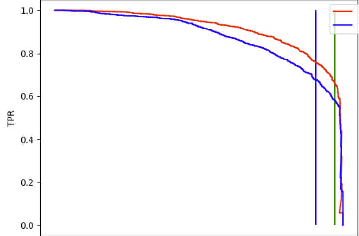
A data scientist may view it is a success: a DL engine that processes tabular data is achieving better results than one of the common ML leading algorithms for such data. However, when we consider real world ML solutions where their requirements are not restricted to the model performances only, but to other questions such as explainability risk and causality, such “desired by data scientists result” may leave some open questions and challenges for the business units and the customers. It is well known that while classical ML algorithms nearly always provide features importance score. DL not only avoid providing such indices but often mask this information.
What are Bayesian Networks?
The motivation of using Bayesian Networks (BN) is to learn the dependencies within a set of random variables. The networks themselves are directed acyclic graphs (DAG) which mimics the joint distribution of the random variables. The graph structure follows the probabilistic dependencies factorization of the joint distribution: a node V depends only on its parents (namely a r.v X which is independent on the other nodes will be presented as a parent free node). A tutorial on this topic can be found here
Steps in BN learning
- Constructing DAG- As we described, the outcome of BN training is a well approximated DAG. This graph aims to illustrate both the dependencies between the variables and the simplest factorization of the joint distribution. Clearly such task is better achieved with the presence of expert knowledge. Namely when some of its arcs are known. As an example if we have a problem that it is obvious that there is a target variable then we can initiate the edges that contain it and let the training mechanism use it as a prior knowledge. There are two main classes of methods for training BN in order to obtain DAG:
Constraint-based structure learning- For understanding this approach we use the following definition:
Markov Blanket- a Markov Blanket of r.v Y is a set A of r.v {X1, …Xn} where for any subset S of A, Y is independent of A\S |S ,namely if we condition the random variables on S we obtain a co-set that is independent of Y.
An algorithm for finding DAG is composed therefore from three stages: Learning Markov Blanket, finding neighbors and determining arc directions. In the first stage we identify the conditional independence between variables using chi score (which is commonly used in t test)
Score based structure learning- This class is more useful practically as it is “considered more promising due to the statistical scoring approach” .
We determine in advance a searching and scoring methods. Defining an initial DAG (that can be the empty one as well). At each step we add, withdrawal or revert an edge and calculate a statistical score. We repeat this process until a convergence is obtained. We seldom have small amount of variables, thus brute force approaches (exhaustive search) are rarely practical. But we can use heuristic algorithms. A common example for such algorithm is the following :
Hill Climbing- Simply define a DAG and run as long as the score is improved.
Another algorithm that is commonly used is Chow Liu tree.
Chow Liu- This algorithm approximates a distribution Q to the unknown joint distribution P upon factorizing KL divergence term ( a similar concept to variational inference) the scoring is clearly relies on log likelihood.
After constructing the DAG, one may wish to optimize its parameters:
- Parameters’ learning- At this stage we assume the DAG’s structure and upon it optimize the joint distribution throughout its conditional components. Practically we can use MLE methods which are combined with Bayesian prior beliefs over the distributions.
When we complete those two steps (Constructing the DAG and learn its parameters). We can perform an inference over the network. Namely determining probabilities upon data inputs (similarly to DL engines in the cases that some of the features are un observed)
Real World Example
In the next session I will present a short study I did using the tabular data of the DL engine that I presented beyond. For this study I installed the python package bnlearn . An outstanding guidance for this library can be found here.
Before we begin I will remark that since this project is commercial, I have masked the variable names, thus they will have meaningless names.
Constructing Our DAG
We begin by finding our optimal DAG.
import bnlearn as bn
DAG = bn.structure_learning.fit(dataframe)
We have now a DAG. It has a set of nodes and an adjacency matrix that can be found as follow:
print(DAG['adjmat'])
The outcome has this form:

Where rows are sources (namely the direction of the arc is from the left column to the elements in the row) and columns are targets (i.e. the header of the column receives the arcs).
When we begin drawing the obtained DAG we got for one set of variables the following image:
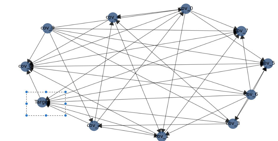
We can see that the target node which is in the rectangle is a source for many nodes. We can see that it still points arrows itself to two nodes. We will discuss this in the discussion section
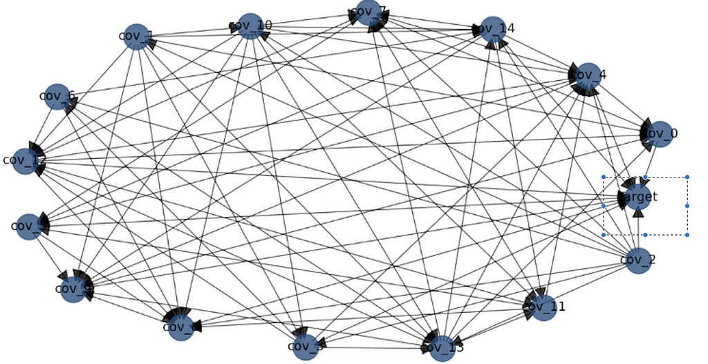
Clearly we have more variables, therefor I increased the amount of nodes.
Adding the information provided a now source fro the target (i.e. its entire row is “False”)
The obtained graph is the following:
So we know how to construct a DAG. Now we need to train its parameters.
Code-wise we perform this as follow:
model_mle = bn.parameter_learning.fit(DAG, dataframe, methodtype='maximumlikelihood')
We can change ‘maximulikelihood’ with ‘bayes’ as described beyond.
The outcome of this training is a set of factorized conditional distributions that reflect the DAG’s structure.
It has this form for a given variable
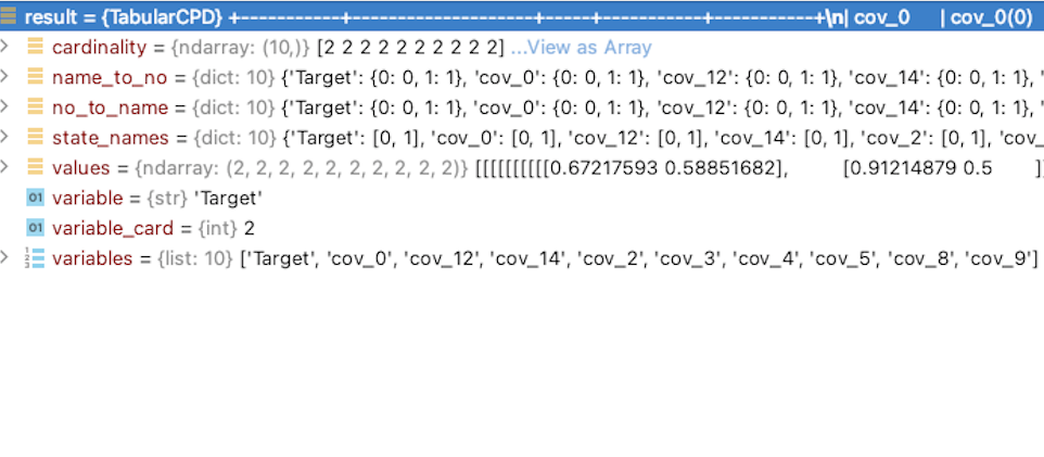
The field “variable” is the name of the node as a target
The field “variables” are its sources
The field “values” is a n- dimensions cube of the conditional probabilities that determine each of the “variable’s” values.
Now we can perform analysis upon this matrix to identify where information (conditional distribution ) exists.
For the inference we decide about the evidence (namely on which of the sources of the target we are conditioning) and we hope to get low conditional entropy
bn.inference.fit(model_mle, variables=['Target'], evidence={'cov_0':0,'cov_1':1 })
The outcome for this line is the following tables:
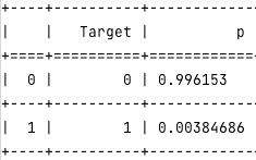
Namely if we condition the target on such values, we can well predict the target outcome.
Discussion
We have presented some of the theoretical concepts of Bayesian networks, and the usage that they provide in constructing an approximated DAG for a set of variables. In addition we presented a real world example of end to end DAG learning: Constructing it using BN, training tis parameters using MLE methods and performing and inference. We may now discuss what is the context of this topic with respect to DL problems. Why are Bayesian networks beneficial for such problems?
Explainability- Obtaining a DAG from a BN training, provides a coherent information about independence variables in the DB. In a generic DL problem, features are functions of these variables. Thus one can derive which of the variables are dominant in our system. When customers or business units are interested in the cause of a neural net outcome, This DAG structure can be both a source to provide importance as well as clarify the model.
- Dimension Reduction — BN provides both the joint distribution of our variables as well as its associations. The latter may play a rile in reducing the features that we induce a DL engine: If we know that for random variables X,Y the conditional entropy of X in Y is low we may omit X since Y provides its nearly entire information. We have therefore a tool that can statistically exclude redundant variables
- Tagging Behavior- This section can be less obvious for those who work in domains such as vision or voice. In some frameworks, labeling can be an obscure task (to illustrate consider a sentiment problem with large number of categories that may overlap). When one tags the data he may rely on some features within the datasets and generate conditional probability. Training BN when we initialize an empty DAG, may provide outcomes in which the target target is a parent of other nodes. Observing several tested examples, these outcomes simply reflect this “taggers’ manners”. We can therefore use DAGs not for ML needs but for learning taggers policy and improve it if needed.
- The conjunction of DL and Casual inference — Causal Inference is an extremely developed domain in data analytics. It offers tools to resolve questions that on one hand DL models commonly not and on the other hand, real world raises. There is a need to find framework in which these tools will work in conjunction. Indeed, such frameworks already exist (e,g. GNN). But a mechanism that merge typical DL problems causality is less common. I believe that flows as described in this post is a good step in the direction of achieving benefits from this conjunction
Acknowledgments
I wish to acknowledge Professor Ziv Bar -Joseph for introducing me this topic and to Uri Itai for fruitful discussions
Explainability Using Bayesian Networks was originally published in Towards Data Science on Medium, where people are continuing the conversation by highlighting and responding to this story.
from Towards Data Science - Medium https://ift.tt/3pRPmOW
via RiYo Analytics

No comments