https://ift.tt/3FbjABb Applying a Machine Learning model to actively test and classify transactions as valid or not Image by author Int...
Applying a Machine Learning model to actively test and classify transactions as valid or not

Introduction
The idea behind the credit card technology actually dates back to the late 1800s, and comes from an utopian novel called Looking Backward, by Edward Bellamy (Wikipedia). However, we’d only begin to see anything like that in the 20th century, but nothing compared to what we have nowadays.
The fact is that credit cards have revolutionized the way we shop and live our lives, without having to walk around with loads of cash on our pockets. It is estimated that, in 2018, a total of 1.2 Billion cards were in circulation only in the US, with 72% of adults having at least one credit card.

Unfortunately, this technology opens up a whole new possibility for scams and frauds. These types os crime happen mostly when data from your card is obtained illegally through various sources, but mostly on database leakages or identity theft schemes (FBI).
However, there are quite many measures you can take in order to prevent having your data stolen. Just to name a few:
- Make sure the website you’re accessing has a valid security certificate;
- Don’t give out your information to anyone you don’t know;
- Don’t believe every product or investment offer you receive via e-mail or on a website.

In order to avoid this kind of fraud, banking companies are always trying to early identify these events, so that the card can be blocked and the transaction fails immediately.
With this in mind, we’ll utilize a dataset available on Kaggle about two days’ worth of transactions from an European bank in 2013, and develop a model to classify transactions as frauds or not.
About our dataset
The raw dataset was composed of 31 attributes (columns), contemplating data about the time, amount and the type of transaction (fraud or not), which will be our target variable. The remaining attributes, for privacy reasons, were treated with the Principal Component Analysis (PCA) method for dimensionality reduction and the description was hidden. As for rows, we have a total of 284407 entries.
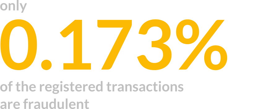
One important aspect about this dataset is its natural imbalance. As expected, we should see many more real transactions than fraudulent ones, and that can be seen within our data. In fact, only 0.173% (492 entries) are classified as frauds.
That actually comes as a problem for our analysis, but we’ll deal with it later on.
Analyzing the distributions
We’ll now take a look at the two main (known) attributes: Amount and Time, in regards to the type of transaction, and begin to analyze our data.
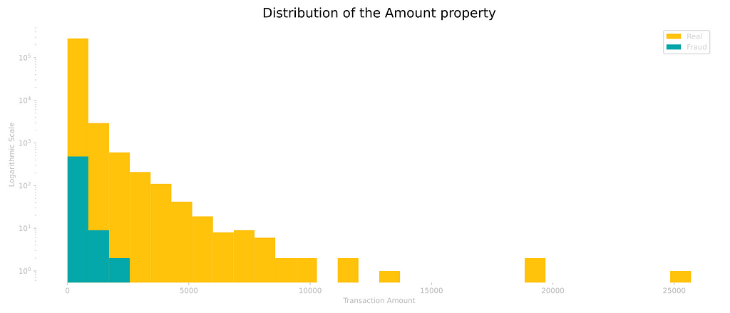
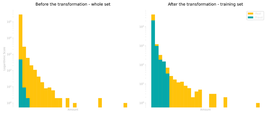
By looking at the Amount property, we can already start to see a few characteristics, such as the fact that the frauds are more common among smaller values.
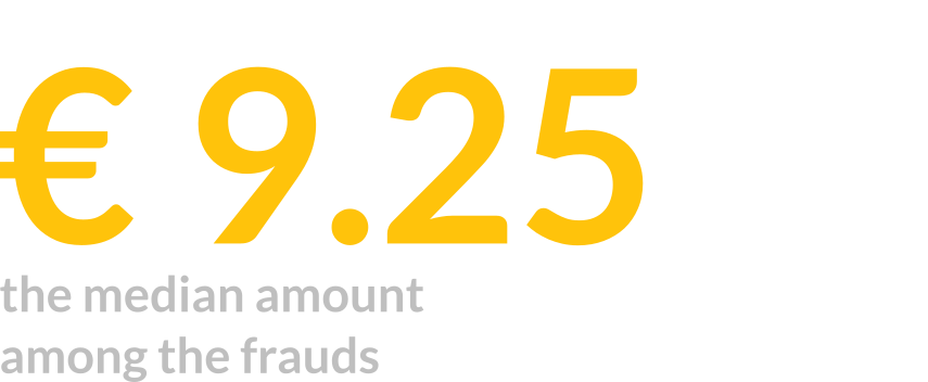
Upon further analysis, it was possible to find the mean amount for the frauds as 122.21 EUR, but with a median of only 9.25 EUR, that is, 50% of all transactions are actually less or equal to the latter amount.
This difference between the median and the mean is actually due to the presence of outliers, entires that don’t fit accordingly into the distribution, bringing the mean to a higher value. The largest fraud recorded actually had an amount of 2125.87 EUR.
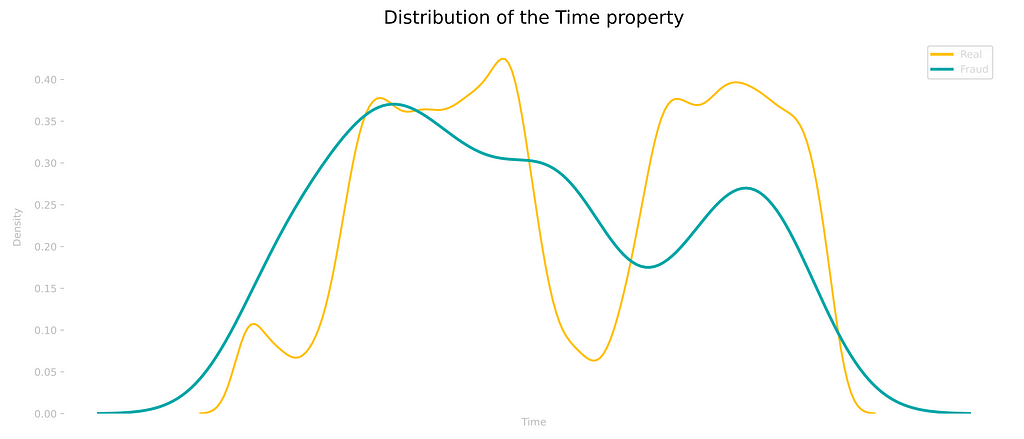
The time property, as we know, relates to 48 hours of transactions. Even though we don’t have the actual time each transaction took place, by looking at the distribution we can draw a few conclusions. The moments we see lower values are, probably, before dawn, when we would expect people not to go around shopping.
However, for the fraudulent transactions, we don’t observe the exact same pattern, as many transactions are actually registered at these periods of the day.
Preparing the dataset
Even though we don’t know the meaning of most of the data, the columns come on a variety of ranges, so the first step will be to adjust these ranges. For that, we’ll standardize the Time and Amount variables, as the rest of the properties have already been treated.
The next step will be to split our dataset between training and testing data, and in X (independent variables) and y (target classes). For this, the chosen test proportion was 20%, with the remaining 80% being assigned to the training set and the values were then randomly distributed.
We still have the imbalance issue to deal with, but we’ll deal with it later for comparison purposes.
Building our Random Forest Classifier
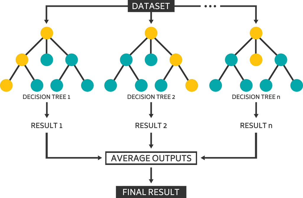
The chosen Machine Learning model for this project was the Random Forest Classifier, from the Scikit-Learn Python library. Random Forests are an upgrade to the common Decision Trees we intuitively use on our everyday lives, when we try to make choices based on different characteristics and a series of true or false statements.
Decision Trees tend to create of series of rules and deal with the entire dataset at a time. Random Forests, however, add a pinch of (you guessed) randomness, by choosing different random features and entries for each of the many decision trees built, and then averaging out the results. This variability of the model theoretically creates more accurate predictions, as the many trees tend to attenuate the individual errors of each one of them.
However, how should we evaluate the performance of our model?
That is an extremely important question, and there isn’t an actual global conclusive answers. It always depends on the model and the characteristics of the data we’re working with.
For our specific case, where we have a set of highly imbalanced data and looking for a binary classification (valid or not), the most appropriate method would be the AUC-ROC (Area Under the Curve of the Receiver Operating Characteristics), a measure that deals with the True Positive Rate (TPR) and False Positive Rate (FPR). You can read more about it here.
But, for a brief explanation, our AUC-ROC score will come as value between 0 and 1, where larger values mean that the model is better at correctly identifying the wanted classes. We’ll also use the prediction and recall parameters for comparison.
Training the raw data
The hyperparameters chosen were the standard values from the model (only setting a random_state for reproducibility), with a total of 100 estimators (decision trees).
After the fitting of the model to the training data, we proceeded to predict the classes on our testing data.
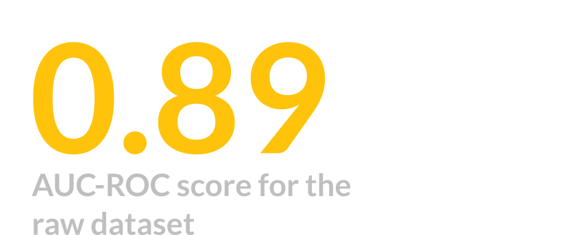
The first model, with the poorly treated data, returned a final score of 0.89, as a predictor with essentially a low false positive rate (precision of 0.92) and a mild false negative rate (recall of 0.78).
Due to the nature of the problem, my approach was to try and minimize the false negative rates, at the expense of eventually increasing the amount of false positive results. The hypothesis is that a preventive blockage (eventual social nuisance) is preferred over a fraudulent transaction passing through, which would cause issues like the necessity of a reimbursement.
Treating the imbalance issue
As we’ve seen, our raw dataset is highly imbalanced, and we have a few techniques to reduce this issue. These techniques can be classified as either oversampling or undersampling methods. In this analysis, we’ll use both, with the methods from the Imbalanced Learn Python library.
As the name suggests, each of these techniques either increases or decreases the number of observations on our dataset. We begin by oversampling with SMOTE (Synthetic Minority Oversampling Technique) for a target proportion of 1:10 (10% total), which essentially creates new entries for the smaller class (frauds), by generating property values that fit within the original observations.
For undersampling, we’ll use the Random Under Sampler method for a proportion of 5:10 (double of the minority class), which randomly picks out some of the largest class (valid) entries and erases them from the dataset.
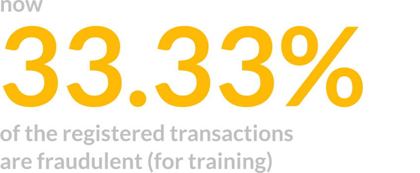
With this, we now have a third of the whole set as frauds. The important thing to point out is that only the training set went through this transformation. We want to keep the testing data as real as it gets, in order to properly evaluate our model.
Below we can see a side-by-side comparison of the distribution before and after treating the imbalance.
We now proceed to create a new model, this time with the more balanced dataset.
Training the new treated data
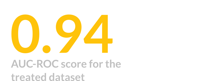
The same hyperparameters were kept for comparison, and now we were able to retrieve an AUC-ROC score of 0.94, 0.5 points higher than the previous model. The desired result was reached, achieving lower false negatives on behalf of more false positives.
Conclusion
In this project, it was possible to identify the Random Forest algorithm as an effective way to classify fraudulent credit card transactions. From a large and imbalanced dataset, we could test the model’s accuracy prior to treating the data and afterwards.
In order to treat the imbalance, 2 techniques were applied to the training set: SMOTE and Random Under Sampling. With them, an original imbalance of 0.17% on the fraudulent transactions was turned into a proportion of 66/33 between the categories.
The main chosen metric to evaluate the model’s performance, the AUC-ROC, was significantly improved from the raw model to the treated one: 0.89 and 0.94 scores, respectively.
The imbalance treatment effectively improved the model’s performance, but also increased the false positive ratio. Due to the problem’s nature, this result is justifiable, as it’s desirable to better detect frauds, on behalf of a few more false positives.
Thanks for the support!
You can access the entire notebook here.
Early Detecting Credit Card Frauds was originally published in Towards Data Science on Medium, where people are continuing the conversation by highlighting and responding to this story.
from Towards Data Science - Medium https://ift.tt/34r8tY3
via RiYo Analytics

No comments