https://ift.tt/3rv1V2p A Guide to Classifying Complex Texts with Transformers By Jaren R Haber (Georgetown University), Thomas Lu (Unive...
A Guide to Classifying Complex Texts with Transformers
By Jaren R Haber (Georgetown University), Thomas Lu (University of California, Berkeley), and Nancy Xu (University of California, Berkeley)

For researchers and scientists, there is too much to read out there: more blog posts, journal articles, books, technical manuals, reviews, etc., etc. than ever before. Yet read we must, for the main way to learn from the past and keep from reinventing the wheel — or worse, the flat tire — is through the time-honored practice of literature review. How can we keep up with the Joneses — that is, the academic state-of-the-art and its many changes over time — when our desks and bookshelves overflow with knowledge, providing far too much content for a human to digest?
To the rescue comes a favorite pastime of the digital age: computers reading things, or natural language processing (NLP). We provide NLP tools and example code to help parse academic journal articles, which are growing exponentially in number — and especially so for interdisciplinary research, which crisscrosses academic fields. As a case study, we develop methods to read and track one specific interdisciplinary area: organizational theory in the disciplines of sociology and management studies. We use deep learning to help read this literature at a large scale, a pipeline we call computational literature review.
We specifically trace the three big perspectives in modern sociology and management studies — demographic, relational, and cultural — in a corpus of about 70,000 journal articles provided by JSTOR. Our models determine which of these perspectives (if any) are used in an academic text by leveraging a powerful suite of NLP tools: pretrained Transformer models. Transformers can process a body of text, “understand” its contents at a high level using attention layers and neural networks, and generate useful output such as predictions. They are a state-of-the-art, nuanced tool for training machine learning classifiers, which we build to help review the academic literature.
After reading this blog, you should be able to:
- Understand our workflow for tracking ideas in digital text corpora, from preprocessing to model training
- Compare the performance of several deep learning algorithms in capturing organizational theories
- Visualize how perspectives shift in academic texts over time
- Locate (and build on!) our code for computational literature review
Workflow
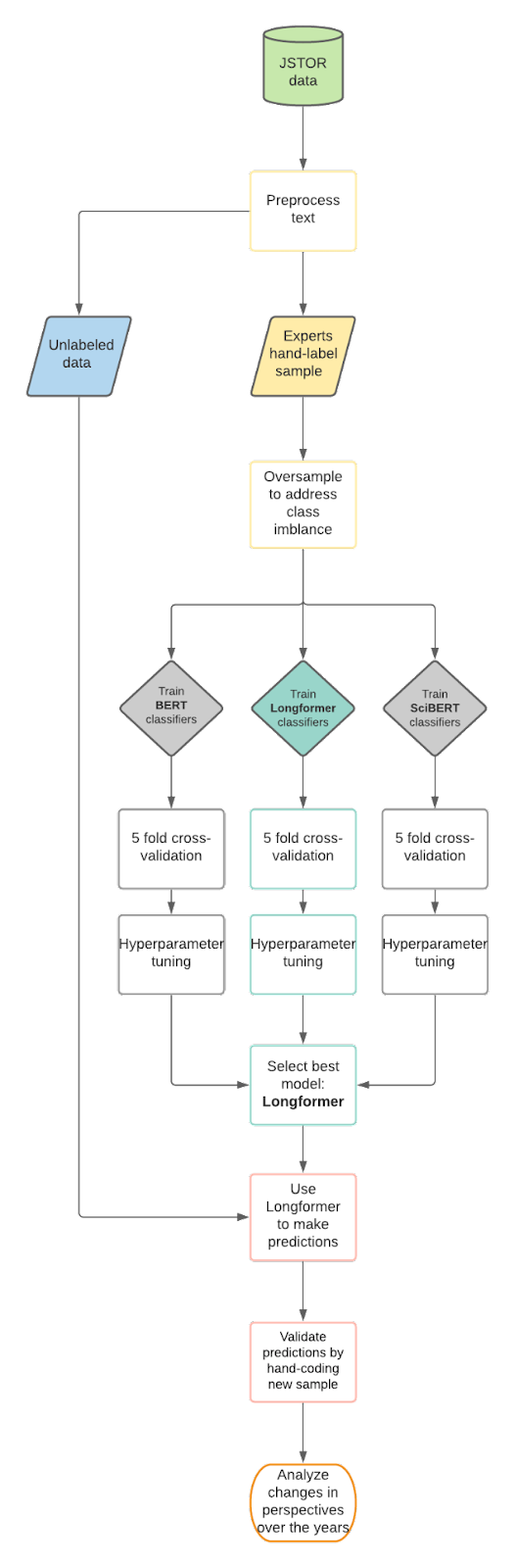
The expert organizational scholars on our team hand-coded about 700 articles to provide ground truth for the presence of each perspective. We use this labeled training data to train Transformer-based classifiers on preprocessed full text data from JSTOR. These models output binary predictions for three perspectives in organizational theory, and we selected the best one based on cross-validation accuracy. Then we make predictions on unlabeled data and analyze trends in each perspective across the disciplines of sociology and management studies.
Our goal is to classify academic articles, which are on average 7640 words in length. However, traditional Transformer-based models are often unable to process long sequences: BERT relies on self-attention, which scales quadratically with sequence length and creates untenable computational demands when processing longer sequences. This limitation is important here, given that often-long articles are our unit of analysis. In addition, BERT is pre-trained on the eBooksCorpus (800M words) and English Wikipedia (2,500M words), which may limit its transferability to our domain of scientific literature. For these reasons, we narrowed our focus to two variations of Transformer models, along with BERT itself for comparison: SciBERT and Longformer. SciBERT is based on BERT but is trained on academic journal articles more similar to our corpus: specifically, its corpus is 1.14M papers from Semantic Scholar (18% from computer science and 82% from biomedical domain).
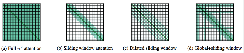
In contrast, Longformer is a Transformer-based model trained on the same original dataset as BERT, but it can take in a maximum of 16K tokens (as opposed to 512 for BERT and SciBERT). Longformer minimizes the computational burdens of attention by performing not all possible comparisons but only those with the relevant words. Longformer provides a number of strategies to do this (see figure below), such as letting most tokens only attend to their neighbors, while only a few attend to every token (and every token also attends to them).
This longer sequence length allows our deep learning classifiers to capture organizational perspectives embedded not only in the Abstract or Introduction of academic articles, but also later in the body of the text (such as the Theory section). We trained Longformer models with a maximum token length of 1024 (for resource management reasons), well below the 16K limit. Even so (spoiler alert), this greater sequence length proved a key advantage for Longformer in our case, yielding a 2% or so improvement in accuracy compared to BERT.
Code for our workflow
Preprocessing
Because Transformers like BERT utilize structures of the sentence and assign meaning to words based on their surrounding words (amounting to a context-unique vector for each word, an advantage over word embeddings like word2vec), stop words and grammatical structures are important for model training. Thus, we preprocess the text minimally, tokenizing the text with the Apache Lucene tokenizer, and removing only HTML tags, page formatting markers, and other miscellaneous junk. The following simple RegEx substitutions clean page formatting and XML tags left over from JSTOR’s digitization of article text with OCR. Our complete text preprocessing code can be found here.
def remove_tags(article):
    """
    Cleans page formatting and XML tags from JSTOR articles.
    """
    article = re.sub(‘<plain_text> <page sequence=”1">’, ‘’, article)
    article = re.sub(r’</page>(\<.*?\>)’, ‘ \n ‘, article)
    # remove xml tags
    article = re.sub(r’<.*?>’, ‘’, article)
    article = re.sub(r’<body.*\n\s*.*\s*.*>’, ‘’, article)
return article
Oversampling
Because our binary classifiers predict only two classes, the best class balance in our training data would be 1:1: 50% true positive cases (perspective is referenced in the article), 50% true negative cases (perspective not referenced). However, our hand-labeled data include about twice as many negative as positive cases. To address this class imbalance in the training and test samples, we oversample by bootstrapping from the minority class (positive cases) to reach a 1:1 class ratio.
from imblearn.over_sampling import RandomOverSampler
from imblearn.under_sampling import RandomUnderSampler

def oversample_shuffle(X, y, random_state=52):
    """
    Oversamples X and y for equal class proportions.
    """

    fakeX = np.arange(len(X), dtype=int).reshape((-1, 1))
    ros = RandomOverSampler(random_state=random_state, sampling_strategy=1.0)
    fakeX, y = ros.fit_resample(fakeX, y)
    p = np.random.permutation(len(fakeX))
    fakeX, y = fakeX[p], y[p]
    X = X.iloc[fakeX.reshape((-1, ))]
return X.to_numpy(), y.to_numpy()
Train-test split
Model training requires separate training and test sets to provide accurate predictions. To create our datasets for training, we perform a train-test split and then oversample both sets to address the class imbalance mentioned earlier.
def create_datasets(texts, scores, test_size=0.2, random_state=42):
    """
    Splits the texts (X variables) and the scores (y variables)
    then oversamples from the minority class to achieve a balanced sample.
    """

    X_train1, X_test1, y_train1, y_test1 = train_test_split(
        texts, scores, test_size=test_size,
        random_state=random_state)
    X_train1, y_train1 = oversample_shuffle(
        X_train1, y_train1, random_state=random_state)
    X_test1, y_test1 = oversample_shuffle(
        X_test1, y_test1, random_state=random_state)

    return X_train1, y_train1, X_test1, y_test1
Model Training
We build our classifier on top of a Longformer model from the HuggingFace Transformers library, as well as a single linear layer to convert the Longformer representations to a set of predictions for each label. Here is the BERTClassifier class that contains code for loading and initializing the pretrained long former model with specified max token length, and helper functions such as `get_batches()`, `forward()`, and `evaluate()` for model training and cross-validation. Here’s the full code for the model training.
class BERTClassifier(nn.Module):
    """
    Initializes the max length of Longformer, the pretrained model, and its tokenizer.
    """
    def __init__(self, params):
        super().__init__()
        self.tokenizer = LongformerTokenizer.from_pretrained('allenai/longformer-base-4096')
        self.bert = LongformerModel.from_pretrained("allenai/longformer-base-4096", gradient_checkpointing=True)
        self.fc = nn.Linear(768, self.num_labels)
We then define the `get_batches()` helper function within the `BERTClassifier` class that tokenizes the text using a BERT tokenizer.
    def get_batches(self, all_x, all_y, batch_size=10):
        """
        Tokenizes text using a BERT tokenizer.
        Limits the maximum number of WordPiece tokens to 1096.
        """
        batch_x = self.tokenizer.batch_encode_plus(
            x, max_length=self.max_length, truncation=True,
            padding='max_length', return_tensors="pt")
batch_y=all_y[i:i+batch_size]
## code omitted
return batches_x, batches_y
To run the model, we define a `forward()` function within `BERTClassifier`. This gets model output and runs the last layer through a fully connected linear layer to generate predictions by performing the softmax of all output categories, as is typical in logit models.
    def forward(self, batch_x):
        """
        Gets outputs from the pretrained model and generates predictions.
        Note that Longformer is a RoBERTa model, so we don't need to pass in input type ids.
        """
        # First, get the outputs of Longformer from the pretrained model
        bert_output = self.bert(input_ids=batch_x["input_ids"],
                        attention_mask=batch_x["attention_mask"],
                        output_hidden_states=True)

        # Next, we represent an entire document by its [CLS] embedding (at position 0) and use the *last* layer output (layer -1).
            bert_hidden_states = bert_output['hidden_states']
            out = bert_hidden_states[-1][:,0,:]
            if self.dropout:
                out = self.dropout(out)
            out = self.fc(out)
return out.squeeze()
Lastly, we define an `evaluate()` function for `BERTClassifier` to determine the accuracy of predictions of batch x based on batch y.
    def evaluate(self, batch_x, batch_y):
        """
        Evaluates the model during training by getting predictions (batch x) and comparing to true labels (batch y).
        """
        self.eval()
        corr = 0.
        total = 0.
        # disable gradient calculation
        with torch.no_grad():
            for x, y in zip(batch_x, batch_y):
        # for each batch of x and y, get the predictions
        # and compare with the true y labels
                y_preds = self.forward(x)
                for idx, y_pred in enumerate(y_preds):
                    prediction=torch.argmax(y_pred)
                    if prediction == y[idx]:
                        corr += 1.
                    total+=1

       return corr/total
We then train the model and determine the best hyperparameters. We used Microsoft Azure’s machine learning servers to search the hyperparameter space and maximize cross-validation accuracy; here is the full code to do this. The workhorse in this code is the `train_bert()` function below, which uses `create_datasets()` to prepare the training and testing data and then `get_batches()` from the `BERTClassifier`class to get batches for model construction. Next, we define the hyperparameter variables, the Adam optimizer, and its scheduler. We then train and evaluate the model, recording its best dev accuracy and epoch for use in model comparison.
def train_bert(texts, scores, params, test_size=0.2):
    """
    This deep learning workhorse function trains a BERT model
    with the given hyperparameters,
    returning the best accuracy out of all epochs.
    (Code is simplified for ease of reading.)
    Inputs:
        texts: a list of article texts for training
        scores: a list of labels for the texts (0 or 1)
        test_size: proportion of input data to use for model testing (rather than training)
        params: a dict of parameters with optional keys like batch_size, learning_rate, adam_beta, weight_decay, max_memory_size, and num_epochs (full list omitted).
    """
    # cross entropy loss is used for binary classification
    cross_entropy=nn.CrossEntropyLoss()
    best_dev_acc = 0.
    best_dev_epoch = 0.
    for epoch in tqdm(range(num_epochs)): # loop over epochs
        bert_model.train()
        # Train model
        optimizer.zero_grad() # Clear any previously accumulated gradients
        for i, (x, y) in enumerate(zip(batch_x, batch_y)):
            # Find the loss for the next training batch
            y_pred = bert_model.forward(x)
            loss = cross_entropy(y_pred.view(-1, bert_model.num_labels), y.view(-1))
            loss.backward() # Accumulate gradients for back-propagation
            if (i + 1) % (batch_size // max_memory_size) == 0:
                # Check if enough gradient accumulation steps occurred. If so, perform a step of gradient descent
                optimizer.step()
                scheduler.step()
                optimizer.zero_grad()

       # Evaluate model and record best accuracy and epoch
        dev_accuracy=bert_model.evaluate(dev_batch_x, dev_batch_y)
        if epoch % 1 == 0:
            if dev_accuracy > best_dev_acc:
                best_dev_acc = dev_accuracy
                best_dev_epoch = epoch

    print("\nBest Performing Model achieves dev accuracy of : %.3f" % (best_dev_acc))
    print("\nBest Performing Model achieves dev epoch of : %.3f" % (best_dev_epoch))
return best_dev_acc
Model Evaluation
We tie together all the above with the `cross_validate()` function, which takes in a list of preprocessed text, a list of their categorical scores (1 if the article is about a given perspective, 0 otherwise), and a list of hyperparameters to tune. This function then trains the model and returns the cross-validation accuracy, or the model’s average accuracy across each of several (here, 5) slices or folds of the data. Compared to a single train/test split, k-fold cross-validation provides a more generalizable measure of model performance, minimizing the risk of model overfitting on input data.
def cross_validate(texts, scores, params, folds=5, seed=42):
    """
    Trains BERT model and returns cross-validation accuracy.
    Communicates directly with Azure to run model
    and record accuracy of given hyperparameters.
    """

    np.random.seed(seed)
    states = np.random.randint(0, 100000, size=folds)
    accs = []
    for state in states:
        print(state)
        accs.append(train_bert(
            texts, scores, params, test_size=round(1/folds, 2),
            random_state=state, save=False))
    acc = np.mean(accs)
    run.log('accuracy', acc) # works with Azure
return acc
Here is an example usage of our code, using the `orgs` Pandas dataframe for training data. Each row is a sociology article, the column `full_text` contains the article’s full text, and `orgs_score` indicates whether the article is about organizations (1) or not (0).
orgs['text_no_tags'] = [remove_tags(art) for art in orgs['full_text']]
orgs = orgs[orgs['orgs_score']!=0.5]

cross_validate(orgs['text_no_tags'], orgs['orgs_score'],{'batch_size': 16, 'lr': 1e-4, 'dropout': 0.2, 'weight_decay':0.005, 'num_warmup_steps': 60})
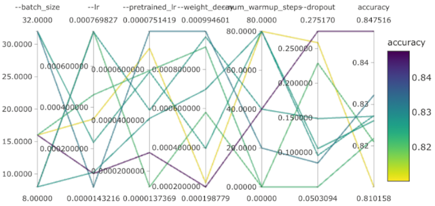
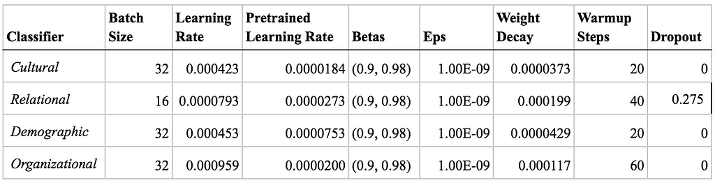
The results can then be visualized using Azure’s specialized machine learning dashboards. The graph below shows the combination of hyperparameters (batch size, learning rate, pretrained learning rate, weight decay, number of warm up steps, and dropout rate) for the models we trained. The most accurate model (purple line) has relatively low values for all hyperparameters except dropout rate.
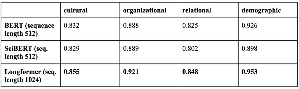
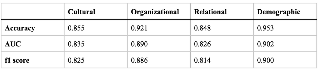
Compared to BERT and SciBERT, we find that optimized binary classifiers built on Longformer perform the best across all three perspectives and organizational sociology. The table below compares the accuracy of the different transformer models we tested. See Appendix A for optimal model hyperparameters and Appendix B for alternative metrics of Longformer’s performance.
Making and visualizing predictions
Due to its superior performance, we used Longformer to generate binary and continuous predictions (yes/no and the probability of engaging each perspective) for the 65K or so yet-unlabeled JSTOR articles. You can find here the full code for generating predictions.
def get_preds(model, batch_x, batch_y):
    """
    Using input model, outputs predictions (1,0) and
    scores (continuous variable ranging from 0 to 1) for batch_x
    Note that batch_y contains dummy labels to take advantage of pre-existing batching code
    """
    model.eval()
    predictions = []
    scores = []
    with torch.no_grad():
        for x, y in tqdm(zip(batch_x, batch_y)):
            y_preds = model.forward(x)
            for idx, y_pred in enumerate(y_preds):
                predictions.append(torch.argmax(y_pred).item())
                sm = F.softmax(y_pred, dim=0)
            try:
                scores.append(sm[1].item())
            except:
                print(len(scores))
                print(sm.shape, sm)
return predictions, scores
We divided the JSTOR corpus into two primary subjects (sociology and management & organizational behavior) and analyzed engagement with each of the three perspectives (demographic, cultural, and relational). We filtered out sociology articles with a predicted probability of being about organizations that is lower than 0.7.
# filter to only organizational sociology articles using threshold of 0.7
minority_threshold_orgs = 0.7
df_orgsoc = merged[merged['primary_subject']=='Sociology'][merged['org_score'] > minority_threshold_orgs]
Next we make a helper function `cal_yearly_prop()` to calculate the annual proportions of articles engaging each perspective. This helps visualize the proportion of articles engaging each perspective over time.
def cal_yearly_prop(df_category):
    """
    For graphing purposes, calculate the proportion of articles
    engaging a perspective (cultural, relational, or demographic)
    for a given discipline (sociology or management studies) over years.
    Arg:
        df_category: DataFrame of article predictions with columns ‘publicationYear’ indicating year published and ‘article_name’ as identifier
    Returns:
        A list of proportion of articles engaging in a perspective over the years
    """

    yearly_grouped = df_category.groupby('publicationYear').count()
    yearly_total = list(yearly_grouped[‘article_name’])
    years = list(yearly_grouped.index)
    # get the yearly counts of articles
    counts = df_category.groupby('publicationYear').count()[['article_name']].reset_index()
    not_present = list(set(years) - set(counts.publicationYear))
    # create a dataframe for the article counts of missing years (0)
    df2 = pd.DataFrame.from_dict({'publicationYear':not_present, 'article_name': [0]*len(not_present)})

    # concatenate the counts df with df of missing years, and divide the yearly counts by yearly total to get a list of yearly proportions
    return np.array(pd.concat([counts, df2]).reset_index().sort_values('publicationYear')['article_name'])/yearly_total
The stacked bar plot plots below show the changes in the proportion of articles in sociology and management over time. The numerator in this metric is the number of articles that engage in either cultural sociology, relational sociology, or demographic sociology in a given year; the denominator is the total number of articles in sociology in that year. The code for visualizing trends in management studies is very similar. You can find here the full code for visualizing predictions.
# Visualize engagement across perspectives in organizational sociology
relt_fig = plt.figure()
relt_fig.set_figwidth(10)
relt_fig.set_figheight(8)

yearly_grouped = df_orgsoc.groupby('publicationYear').count()
years = list(yearly_grouped.index)

ax = plt.gca()
# the start and end years are omitted because they are outliers
demog_fig = plt.bar(years[1:-1], demog_soc_minority_prop_os[1:-1], color = 'yellowgreen')
cult_fig = plt.bar(years[1:-1], cult_soc_minority_prop_os[1:-1], bottom = demog_soc_minority_prop_os[1:-1], color = 'gold')
relt_fig = plt.bar(years[1:-1], relt_soc_minority_prop_os[1:-1], bottom =  demog_soc_minority_prop_os[1:-1] + cult_soc_minority_prop_os[1:-1], color = 'lightblue')

plt.legend([ 'demog_soc','cult_soc', 'relt_soc' ])

plt.title('Changes in Proportion of Articles in Organizational Sociology from 1971 - 2015')
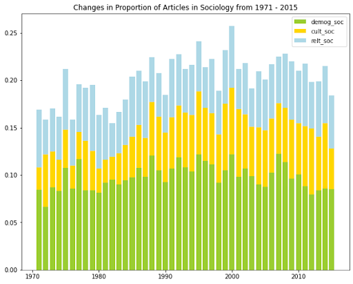
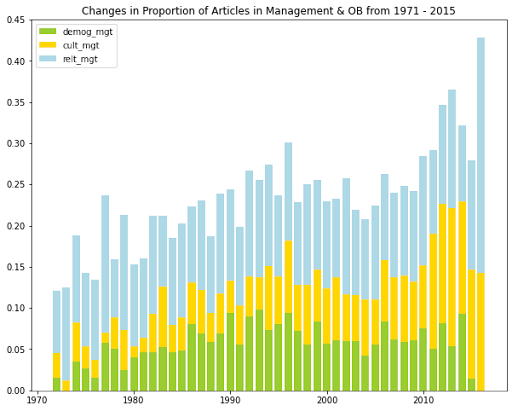
In brief, we see that the demographic perspective was the most common in articles in (organizational) sociology, while the relational perspective was the most common in management and organizational behavior. Demographic management articles gradually declined starting in 2010, and cultural management articles gradually grew over the observed time period. All other categories fluctuated over the years but exhibited no general growth nor decline over time.
Conclusion
We hope that you enjoyed learning about our deep learning workflow for tracking changing ideas in complex texts over time, as applied to our case study of organizational theory in academic articles. To review: We prepare an entire corpus of published literature, use several transformer models to analyze and predict article content, and then chart engagement with specific theories across time and disciplines. Our overall goal is to increase the accessibility of literature review by using data science tools to read and interpret large bodies of text. We think transformers are a great fit for this application, motivating our technical insights into applying transformers to academic articles in various social science disciplines — an exercise we haven’t seen before.
We hope you found our demonstration to be interesting and useful for your own work. Keep an eye out for our future work exploring other sampling methods, model validation with hand-coding, and longer sequence lengths (see Appendix C for specific thoughts on this). We also plan to analyze citation patterns and the changing lexica representing perspectives in organizational theory. Please look forward to it, and thanks for reading!
Appendix
A. Best Model Hyperparameters
As another method of increasing input sequence length, we also explored the “chunking” technique with BERT: We split the text into smaller portions, evaluated the model on each chunk, and combined the results (reference). We found no significant differences between chunking with BERT and using its default sequence length of 512 tokens.
B. Alternative Longformer Metrics
C. Future Work
Model Validation with Hand-Coding
To validate our models, we used likelihood thresholds to select six sets of samples (three perspectives across two disciplines), including both the minority and majority classes as well as those with low-confidence predictions (for possible active learning applications). Hand-coding of these samples by our expert collaborators will serve to validate the models, ensuring that past experiences with abundant false positives are not repeated.
Stratified Sampling
During data preprocessing, in addition to oversampling the minority class, it might be beneficial to use stratified sampling. In general, the number of total JSTOR articles that engage our perspectives increased steadily from 1970 to 2005, peaked in 2005, and started to decline sharply from 2005 to 2016. The changes observed in the frequency and proportion of articles above could be due to certain journals changing the number of articles being published, in addition to the potential changes in the perspectives. To ensure certain perspectives are represented in the sample, the population of JSTOR articles could be divided into subpopulations based on characteristics like year and journal of publication. However, this is also dependent on the quantity of articles that JSTOR provides.
Long Model Input Length
Due to time constraints and computation limitations, we trained Longformers with max token length = 1024. However, it would be insightful to continue training Longformers with larger token lengths and observe any changes in accuracy. Cutting out the middle part of a long text (reference) could also be worth exploring. Additionally, during preprocessing, we could also remove the abstract or the metadata information such as author names and emails at the beginning.
Deep Learning Reviews the Literature was originally published in Towards Data Science on Medium, where people are continuing the conversation by highlighting and responding to this story.
from Towards Data Science - Medium https://ift.tt/3tHk2VF
via RiYo Analytics


ليست هناك تعليقات