https://ift.tt/32H06XT Data Manipulation in SQL, Python and R — a comparison A complete and friendly overview of the most common SQL state...
Data Manipulation in SQL, Python and R — a comparison
A complete and friendly overview of the most common SQL statements and their counterparts written in pandas (Python) and dplyr (R)

Table of contents
- Introduction
- CREATE TABLE
- INSERT INTO
3.1 Insert a single observation
3.2 Insert multiple observations - SELECT
4.1 Select all rows and columns
4.2 Select a limited number of rows
4.3 Select specific columns
4.4 SELECT DISTINCT - WHERE condition (filtering)
5.1 One filtering condition
5.2 Multiple filtering conditions - ORDER BY
6.1 Order by one column
6.2 Specify ascending vs. descending order
6.3 Order by multiple columns - Aggregate functions
7.1 COUNT
7.2 AVG, MIN, MAX, …
7.3 Aggregate functions and WHERE condition
7.4 Bonus: DESCRIBE and SUMMARY - GROUP BY
- UPDATE / ALTER TABLE
9.1 Modify the values of an existing column
9.2 Add a new column
9.3 DROP COLUMN - JOIN
10.1 INNER JOIN
10.2 LEFT JOIN
10.3 RIGHT JOIN
10.4 FULL JOIN - Conclusions
- References
1. Introduction
The purpose of this post is to share the most commonly used SQL commands for data manipulation and their counterparts in both Python and R languages.
By providing practical examples, we also want to underline the similarities, both logical and syntactical, between the two different languages.
For the SQL statements, we employ PostgreSQL, a popular open source relational database management system. For Python, we use the pandas¹ library, while for R we exploit the dplyr² package.
Why pandas:
- De facto standard to manage tabular data structures in Python.
- A complete set of out-of-the-box methods for data manipulation.
- Fast and efficient DataFrame³ object.
- Excellent data representation.
Why dplyr:
- Cleaner and more readable code: function chaining by means of the pipe operator %>% allows easier reading and writing of R code, and provides semantic relief.
- Simple and efficient syntax.
- Speed: faster than base R or plyr.
This post is organized in subparagraph by SQL commands⁴, implying SQL as logical entry point. Nevertheless, it can be easily read from other perspectives too, depending on the familiarity with each language.
2. CREATE TABLE
We can create a SQL table with the CREATE TABLE instruction:
CREATE TABLE IF NOT EXISTS customer_table (
 id SERIAL PRIMARY KEY,
 age NUMERIC NOT NULL,
 gender VARCHAR NOT NULL
);
The pandas equivalent for a SQL table is the pandas.DataFrame, an object that can store two-dimensional tabular data. It can be created as follows:
# the pandas library is imported first
import pandas as pd
columns = {'id':int(),
           'age':int(),
           'gender':str()}
customer_table = pd.DataFrame(columns, index=[])
R provides a data frame as well, and it can be created through the base data.frame()⁵ function:
# the dplyr package is imported first
library(dplyr)
customer_table <- data.frame(id=integer(),
                             age=integer(),
                             gender=character())
3. INSERT INTO
3.1 Insert a single observation
Once we have created the data structures, either tables or data frames:
- We can add rows to the SQL table through the INSERT INTO⁴ statement.
- We can add rows to a pandas.DataFrame with the pandas.DataFrame.append()⁶ method.
- We can add rows to a R data frame with the add_row()⁷ function.
SQL statement:
INSERT INTO customer_table VALUES
  (1, 27, 'Female');
Python:
customer_table = customer_table.append(
   {'id': 1, 'age': 27, 'gender': 'Female'},
   ignore_index=True)
R:
customer_table <-
  customer_table %>% add_row(id=1, age=27, gender='Female')
Note: when we created the pandas DataFrame, we specified column data types. Nevertheless, one may add a record with a different data type from the one originally specified for a column, and no error would be raised.
For example, this Python statement is perfectly valid, even if we previously specified that gender is of type string:
customer_table = customer_table.append(
   {'id': 1, 'age': 27, 'gender': 2})
type(customer_table['gender'].values[0])
# prints: 'int'
3.2 Insert multiple observations
SQL statement:
INSERT INTO customer_table VALUES
  (1, 27, 'Female'),
  (2, 27, 'Female'),
  (3, 45, 'Female'),
  (4, 18, 'Male'),
  (5, 23, 'Male'),
  (6, 43, 'Female'),
  (7, 28, 'Female'),
  (8, 27, 'Male'),
  (9, 19, 'Male'),
  (10, 21, 'Male'),
  (11, 24, 'Male'),
  (12, 32, 'Female'),
  (13, 23, 'Male');
Python:
customer_table = customer_table.append([
   {'id': 1, 'age': 27, 'gender': 'Female'},
   {'id': 2, 'age': 27, 'gender': 'Female'},
   {'id': 3, 'age': 45, 'gender': 'Female'},
   {'id': 4, 'age': 18, 'gender': 'Male'},
   {'id': 5, 'age': 23, 'gender': 'Male'},
   {'id': 6, 'age': 43, 'gender': 'Female'},
   {'id': 7, 'age': 28, 'gender': 'Female'},
   {'id': 8, 'age': 27, 'gender': 'Male'},
   {'id': 9, 'age': 19, 'gender': 'Male'},
   {'id': 10, 'age': 21, 'gender': 'Male'},
   {'id': 11, 'age': 24, 'gender': 'Male'},
   {'id': 12, 'age': 32, 'gender': 'Female'},
   {'id': 13, 'age': 23, 'gender': 'Male'}])
R:
id_list <- c(2, 3, 4, 5, 6, 7, 8, 9, 10, 11, 12, 13)
age_list <- c(27, 45, 18, 23, 43, 28, 27, 19, 21, 24, 32, 23)
gender_list <- c("Female", "Female", "Male", "Male", "Female",
                 "Female", "Male", "Male", "Male", "Male", "Female",
                 "Male")
customer_table <-
  customer_table %>% add_row(id = id_list,
                             age = age_list,
                             gender = gender_list)
4. SELECT
4.1 Select all rows and columns
Once we have populated our data structures, we can query them:
- We can select all rows and columns from the SQL table with SELECT *⁴.
- In both Python and R, in order to display all rows and columns one can simply prompt the name of the data frame.
SQL statement:
SELECT *
FROM customer_table;
Output:
 id | age | gender
— — + — — + — — — —
 1  | 27  | Female
 2  | 27  | Female
 3  | 45  | Female
 4  | 18  | Male
 5  | 23  | Male
 6  | 43  | Female
 7  | 28  | Female
 8  | 27  | Male
 9  | 19  | Male
 10 | 21  | Male
 11 | 24  | Male
 12 | 32  | Female
 13 | 23  | Male
(13 rows)
Python, R:
customer_table
4.2 Select a limited number of rows
- In SQL, we can use theLIMIT⁴ clause to specify the number of rows to return.
- The head() function allows to return the number of top rows to display, even if with a slightly different syntax in Python⁸ and R⁹.
- Moreover, in both Python and R it is possible to specify the number of rows to return by specifying index locations.
SQL statement:
--top 3 rows
SELECT *
FROM customer_table
LIMIT 3;
Output:
  id | age  | gender
 — — + — — -+ — — — —
 1   | 27   | Female
 2   | 27   | Female
 3   | 45   | Female
(3 rows)
Python:
# top 3 rows with head
customer_table.head(3)
# top 3 rows by index with iloc
customer_table.iloc[0:3,]
R:
# top 3 rows with head
head(customer_table, 3)
# top 3 rows by index
customer_table[0:3,]
4.3 Select specific columns
SQL statement:
SELECT age, gender
FROM customer_table
LIMIT 3;
Output:
age | gender
 — -+ — — — —
 27 | Female
 27 | Female
 45 | Female
(3 rows)
In both Python and R, columns can be selected either by name or by index position.
Remarks:
- In Python, column names should be specified in double square brackets to return a pandas.DataFrame object. Otherwise, a pandas.Series object is returned.
- Python starts counting indexes from 0, while R from 1. For example, the second column has index 1 in Python and 2 in R.
Python:
# select columns by name
customer_table[['age', 'gender']].head(3)
# select columns by index
customer_table.iloc[:, [1, 2]]
R:
# select columns by name
customer_table[, c('age', 'gender')]
# select columns by index
customer_table[, c(2, 3)]
# dplyr
customer_table %>%
   select(age, gender)
4.4 SELECT DISTINCT
- SELECT DISTINCT allows to return only distinct (different) values in SQL.
- We can achieve the same result in Python by calling the pandas.DataFrame.drop_dupicates()¹⁰ method on a DataFrame, or by applying the distinct()¹¹ function from dplyr in R.
SQL statement:
SELECT DISTINCT age, gender
FROM customer_table;
Output:
age | gender
 — -+ — — — —
 32 | Female
 28 | Female
 45 | Female
 27 | Female
 43 | Female
 23 | Male
 21 | Male
 18 | Male
 24 | Male
 27 | Male
 19 | Male
(11 rows)
Python:
customer_table.drop_duplicates()
customer_table[['age', 'gender']].drop_duplicates()
R:
distinct(customer_table)
customer_table[, c('age', 'gender')]
5. WHERE condition (filtering)
- The WHERE⁴ clause can be used to filter rows based on a specific condition.
- In Python, we can pass this condition inside the pandas.DataFrame.iloc¹² method. The condition will return a boolean array, where True will indicate the indexes of rows matching the condition. Subsequently, iloc will filter the pandas.DataFrame by using the boolean array as input.
- In R, we can make use of the pipe operator %>% and the filter()² method.
5.1 One filtering condition
SQL statement:
SELECT *
FROM customer_table
WHERE gender='Female';
Output:
id  | age | gender
- — + — — + — — — —
 1  | 27  | Female
 2  | 27  | Female
 3  | 45  | Female
 6  | 43  | Female
 7  | 28  | Female
 12 | 32  | Female
(6 rows)
Python:
customer_table.loc[customer_table['gender']=='Female']
R:
customer_table %>% filter(gender=='Female')
5.2 Multiple filtering conditions
SQL statement:
SELECT *
FROM customer_table
WHERE gender='Female' AND age>30;
Output:
  id | age | gender
 — — + — — + — — — —
   3 | 45  | Female
   6 | 43  | Female
  12 | 32  | Female
(3 rows)
Python:
customer_table.loc[(customer_table['gender']=='Female') & (customer_table['age']>30)]
R:
customer_table %>% filter(gender=='Female' & age>30)
6. ORDER BY
- The ORDER BY⁴ command is used to sort the result set in ascending or descending orde,r based on the value of one or multiple columns. By default, it sorts the rows in acending order.
- In Python, we can sort the results with pandas.DataFrame.sort_values()³ , while in R the arrange()¹⁴ function can be used. For both Python and R the default ordering condition is ascending.
6.1 Order by one column
SQL statement:
SELECT *
FROM customer_table
ORDER BY age;
Output:
  id | age | gender
 — — + — — + — — — —
 4   | 18  | Male
 9   | 19  | Male
 10  | 21  | Male
 13  | 23  | Male
 5   | 23  | Male
 11  | 24  | Male
 1   | 27  | Female
 2   | 27  | Female
 8   | 27  | Male
 7   | 28  | Female
 12  | 32  | Female
 6   | 43  | Female
 3   | 45  | Female
(13 rows)
Python:
# default ascending order
customer_table.sort_values(by='age')
R:
# default ascending order
customer_table %>% arrange(age)
6.2 Specify ascending vs. descending order
In SQL, the order can be specified with the DESC (descending) and ASC (ascending) keywords as follows:
SELECT *
FROM customer_table
ORDER BY age DESC;
Output:
 id | age | gender
— — + — — + — — — —
 3  | 45  | Female
 6  | 43  | Female
 12 | 32  | Female
 7  | 28  | Female
 1  | 27  | Female
 2  | 27  | Female
 8  | 27  | Male
 11 | 24  | Male
 13 | 23  | Male
 5  | 23  | Male
 10 | 21  | Male
 9  | 19  | Male
 4  | 18  | Male
(13 rows)
In Python, we can set the ascending property to False for descending order:
customer_table.sort_values(by='age', ascending=False)
R:
customer_table %>% arrange(desc(age))
6.3 Order by multiple columns
SQL statement:
SELECT *
FROM customer_table
ORDER BY age DESC, id DESC;
Output:
 id  | age | gender
 — — + — — + — — — —
 3  | 45   | Female
 6  | 43   | Female
 12 | 32   | Female
 7  | 28   | Female
 8  | 27   | Male
 2  | 27   | Female
 1  | 27   | Female
 11 | 24   | Male
 13 | 23   | Male
 5  | 23   | Male
 10 | 21   | Male
 9  | 19   | Male
 4  | 18   | Male
(13 rows)
Python:
customer_table.sort_values(by=['age', 'id'],
                           ascending=[False, False])
R:
customer_table %>% arrange(desc(age, id))
7. Aggregate functions
7.1 COUNT
SQL statement:
SELECT count(*)
FROM customer_table;
Output:
count
— — — -
13
(1 row)
In Python, we can leverage the pandas.DataFrame.shape method, returning a tuple of size 2 (rows x columns), as well as other approaches:
customer_table.shape[0]
# a less efficient alternative to shape
len(customer_table.index)
In R, we can achieve a similar outcome with the use of nrow or count:
nrow(customer_table)
# as alternative to 'nrow', one may use 'count' from dplyr
count(customer_table)
7.2 AVG, MIN, MAX, …
- SQL supports a plethora of aggregated functions to derive immediately useful information from columns, such as average (AVG), count (COUNT), standard deviation (STDDEV) and more.
- Both Python and R support provide out-of-the-box methods to calculate such metrics.
SQL statement:
-- AVG used as example, other functions include: MIN, MAX, STDEV, …
SELECT AVG(age)
FROM customer_table;
The result can also be rounded to the nth decimal with the ROUND function:
SELECT ROUND(AVG(age), 2)
FROM customer_table;
Output:
-- without ROUND
avg
— — — — — — — — — — -
27.4615384615384615
(1 row)
-— with ROUND
round
— — — -
27.46
(1 row)
Python:
customer_table['age'].mean()
# round the result to the nth decimal
customer_table['age'].mean().round(2)
R:
customer_table %>% summarize(mean(age))
# round the result to the nth decimal
customer_table %>% summarize(round(mean(age), 2))
7.3 Aggregate functions and WHERE condition
SQL statement:
SELECT ROUND(AVG(age),2)
FROM customer_table
WHERE gender='Female';
Output:
round
— — — -
33.67
(1 row)
Python:
customer_table.loc[customer_table['gender']=='Female']['age'].mean().round(2)
In R, it is where multiple operations must be performed that the chaining capabilities of dplyr truly shine:
customer_table %>%
  filter(gender=='Female') %>%
  summarize(round(mean(age), 2))
7.4 Bonus: DESCRIBE and SUMMARY
Python and R provide methods to visualize summary statistics for data frames and their structures.
For example, the pandas.DataFrame.describe()¹⁵ method provides useful insights over numeric columns (non-numeric columns are omitted from the output):
customer_table.describe().round(2)
Output:
      | id    | age
— — — + — — — + — — — —
count | 13.00 | 13.00
mean  | 6.50  | 27.50
std   | 3.61  | 8.66
min   | 1.00  | 18.00
25%   | 3.75  | 22.50
50%   | 6.50  | 25.50
75%   | 9.25  | 29.00
max   | 12.00 | 45.00
count | 12.00 | 12.00
mean  | 6.50  | 27.50
The same method, pandas.Series.describe(), can be also applied only to specific columns (pandas.Series) of interest:
customer_table['age'].describe().round(2)
In R, instead, we can use the summary¹⁶ function to achieve a similar result:
# summary statistics of the whole dataset
summary(customer_table)
# summary statistics of a specific column
summary(customer_table['age'])
Although these native methods are unavailable in standard SQL, one can write queries to achieve similar output. For example:
SELECT
 COUNT(age),
 ROUND(AVG(age),2) AS avg,
 MIN(age),
 MAX(age),
 ROUND(STDDEV(age),2) AS stddev
FROM
 customer_table;
Output:
count | avg   | min | max | stddev
— — — + — — — + — — + — — + — — — —
13    | 27.46 | 18  | 45  | 8.29
(1 row)
8. GROUP BY
The GROUP BY⁴ command allows you to arrange the rows in groups.
SQL statement:
SELECT gender, count(*)
FROM customer_table
GROUP BY gender;
Output:
gender  | count
— — — — + — — — -
Female  | 6
Male    | 7
(2 rows)
In Python, one could use, for example:
1. the pandas.Series.value_counts()¹⁷ method to return the counts of unique values of a feature.
2. the pandas.DataFrame.groupby()¹⁸ method to group data over a feature and perform aggregate operations.
# return unique gender values (Male, Female) and respective counts
customer_table['gender'].value_counts()
# return average age grouped by gender
customer_table.groupby(['gender'])['age'].mean().round(2)
In R, we can leverage the convenient group_by¹⁹ from dplyr to group data, and then calculate metrics through the summarize²⁰ method:
# return both count and average age grouped by gender
customer_table %>%
  group_by(gender) %>%
  summarize(count=n(), round(mean(age), 2))
Output:
gender  | count  | round(mean(age),2)
— — — — + — — — -+ - - - - - - - - - -
Female  | 6      | 33.67
Male    | 7      | 22.14
(2 rows)
9. UPDATE / ALTER TABLE
In SQL, the ALTER TABLE statement is used to add, delete, or modify columns and constraints in an existing table, while the UPDATE statement is used to modify existing records.
9.1 Modify the values of an existing column
SQL statement:
UPDATE customer_table
SET gender = 'M'
WHERE gender = 'Male';
SELECT * FROM customer_table;
Output:
id  | age | gender
 —  + — — + — — — —
 1  | 27  | Female
 2  | 27  | Female
 3  | 45  | Female
 6  | 43  | Female
 7  | 28  | Female
 12 | 32  | Female
 4  | 18  | M
 5  | 23  | M
 8  | 27  | M
 9  | 19  | M
 10 | 21  | M
 11 | 24  | M
 13 | 23  | M
(13 rows)
In Python, we can use the pandas.DataFrame.replace()²¹ method to update the values of an existing column:
customer_table.replace('Male', 'M')
We may also replace multiple values at the same time:
customer_table.replace(['Male', 'Female'], ['M', 'F'] )
In R, we can use mutate()²² as follows:
customer_table %>%
 mutate(gender = case_when(gender == 'Male' ~ 'M',
                           gender == 'Female' ~ 'F'))
9.2 Add a new column
SQL statement:
-- create new column
ALTER TABLE customer_table
ADD COLUMN age_bins VARCHAR;
-- populate column based on existing values
UPDATE customer_table
SET
 age_bins = CASE
 WHEN age < 20 THEN 'Teenager'
 WHEN age > 20 AND age < 30 THEN 'Between 20 and 30'
 WHEN age > 30 AND age < 40 THEN 'Over 30'
 WHEN age > 40 THEN 'Over 40'
 ELSE 'Unknown'
 END;
-- observe result
SELECT * FROM customer_table;
Output:
 id | age | gender  | age_bins
 — —+ — — + — — — — + — — — — — — — — — -
 1  | 27  | Female  | Between 20 and 30
 2  | 27  | Female  | Between 20 and 30
 3  | 45  | Female  | Over 40
 6  | 43  | Female  | Over 40
 7  | 28  | Female  | Between 20 and 30
 12 | 32  | Female  | Over 30
 4  | 18  | Male    | Teenager
 5  | 23  | Male    | Between 20 and 30
 8  | 27  | Male    | Between 20 and 30
 9  | 19  | Male    | Teenager
 10 | 21  | Male    | Between 20 and 30
 11 | 24  | Male    | Between 20 and 30
 13 | 23  | Male    | Between 20 and 30
(13 rows)
In Python, we can achieve this result through the pandas.DataFrame.apply()²³ function, that executes a function along an axis (axis=0 applies the function to each column, whileaxis=1 applies the function to each row) of the pandas.DataFrame:
def age_bins(row):
 if row['age'] < 20:
   return 'Teenager'
 elif row['age'] > 20 and row['age'] < 30:
   return 'Between 20 and 30'
 elif row['age'] > 30 and row['age'] < 40:
   return 'Over 30'
 elif row['age’] > 40:
   return 'Over 40'
 else:
   return 'Unknown'
customer_table['age_bins'] = customer_table.apply(lambda row: age_bins(row), axis=1)
In R, we can still use the mutate function:
customer_table %>%
 mutate(age_bins = case_when(
     age < 20 ~ 'Teenager',
     age > 20 & age < 30 ~ 'Between 20 and 30',
     age > 30 & age < 40 ~ 'Between 30 and 40',
     age > 40 ~ 'Over 40',
     TRUE ~ 'Unknown'))
9.3 DROP COLUMN
- In SQL, we can remove a column from a table through the ALTER TABLE .. DROP COLUMN command.
- In Python, we can simply provide the column names as a list to the pandas.DataFrame.drop()²⁵ method.
- In R, the select()²⁶ function allows to select column by names, where can subtract the column to drop.
SQL statement:
ALTER TABLE customer_table
DROP COLUMN age_bins;
Python:
customer_table.drop(['age_bins'], axis=1)
R:
select(customer_table, -'age_bins')
10. JOIN
Let us assume to have information spread on multiple tables. For instance, we might have a customer table and a purchase table, and we may want to retrieve information across the two table in order to produce a busineess report.
In SQL, we make use of theJOIN⁴ table operator, that allows to combine information from two (or more) tables based on a related column between them.
Before observing the different join conditions, we should create a second table / data frame to experiment with.
SQL statement:
-- create purchase table
CREATE TABLE IF NOT EXISTS purchase_table (
    purchase_id SERIAL PRIMARY KEY,
    product_id VARCHAR NOT NULL,
    price NUMERIC NOT NULL,
 customer_id NUMERIC NOT NULL
);
-- populate purchase table with values
INSERT INTO purchase_table VALUES
  (1, 'SX145', 59.99, 1),
  (2, 'DE438', 19.99, 2),
  (3, 'TG671', 39.99, 4),
  (4, 'ZR565', 129.99, 8),
  (5, 'PO876', 200.00, 5),
  (6, 'LI657', 25.50, 12),
  (7, 'VF455', 69.99, 8),
  (8, 'WS130', 75.00, 8),
  (9, 'CV761', 120.00, 7);

-- observe table
SELECT * FROM purchase_table;
Output:
purchase_id  | product_id | price  | customer_id
-------------+------------+--------+-------------
           1 | SX145      |  59.99 |           1
           2 | DE438      |  19.99 |           2
           3 | TG671      |  39.99 |           4
           4 | ZR565      | 129.99 |           8
           5 | PO876      | 200.00 |           5
           6 | LI657      |  25.50 |          12
           7 | VF455      |  69.99 |           8
           8 | WS130      |  75.00 |           8
           9 | CV761      | 120.00 |           7
(9 rows)
We create the pandas.DataFrame corresponding to the new table:
purchase_table =pd.DataFrame({
    'purchase_id':[1, 2, 3, 4, 5, 6, 7, 8, 9],
    'product_id':['SX145', 'DE438', 'TG671', 'ZR565', 'PO876',
                  'LI657', 'VF455', 'WS130', 'CV761'],
    'price':[59.99, 19.99, 39.99, 129.99, 200.00, 25.50,
             69.99, 75.00, 120.00],
    'customer_id':[1, 2, 4, 8, 5, 12, 8, 8, 7]
})
Similarly, we create a data.framein R:
purchase_table <- data.frame(
  purchase_id = c(1, 2, 3, 4, 5, 6, 7, 8, 9),
  product_id= c('SX145', 'DE438', 'TG671', 'ZR565','PO876','LI657',
                'VF455', 'WS130', 'CV761'),
  price = c(59.99, 19.99, 39.99, 129.99, 200.00, 25.50,
            69.99, 75.00, 120.00),
  customer_id = c(1, 2, 4, 8, 5, 12, 8, 8, 7))
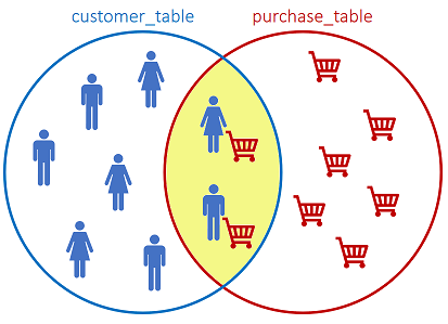
10.1 INNER JOIN
The INNER JOIN returns records that have matching values in both tables, based on a related column:
SQL statement:
SELECT *
FROM customer_table as customer
 INNER JOIN purchase_table as purchase
   ON customer.id = purchase.customer_id;
Output:
id | age | gender | purchase_id | product_id | price  | customer_id
---+-----+--------+-------------+------------+--------+-------------
 1 |  27 | Female |           1 | SX145      |  59.99 |           1
 2 |  27 | Female |           2 | DE438      |  19.99 |           2
 4 |  18 | Male   |           3 | TG671      |  39.99 |           4
 5 |  23 | Male   |           5 | PO876      | 200.00 |           5
 7 |  28 | Female |           9 | CV761      | 120.00 |           7
 8 |  27 | Male   |           4 | ZR565      | 129.99 |           8
 8 |  27 | Male   |           7 | VF455      |  69.99 |           8
 8 |  27 | Male   |           8 | WS130      |  75.00 |           8
 12|  32 | Female |           6 | LI657      |  25.50 |          12
(9 rows)
We have 13 customers and 9 purchases. As the INNER JOIN only returns matching values, we only observe 9 records. The customers that have not performed a purchase are not returned by the query.
In Python, we can use pandas.DataFrame.merge()²⁷ as follows:
pd.merge(customer_table,
  purchase_table,
  left_on='id',
  right_on='customer_id')
By default, pandas.DataFrame.merge() performs an INNER JOIN.
In R, we can make use of the dplyr join methods²⁸:
customer_table  %>%
    inner_join(purchase_table, by=c('id' = 'customer_id'))
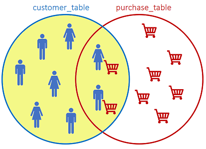
10.2 LEFT JOIN
The LEFT JOIN returns all records from the left table, and the matched records from the right table:
SQL statement:
SELECT *
FROM customer_table as customer
  LEFT JOIN purchase_table as purchase
    ON customer.id = purchase.customer_id;
Output:
 id | age | gender | purchase_id | product_id | price  | customer_id
----+-----+--------+-------------+------------+--------+------------
  1 |  27 | Female |           1 | SX145      |  59.99 |           1
  2 |  27 | Female |           2 | DE438      |  19.99 |           2
  3 |  45 | Female |             |            |        |
  4 |  18 | Male   |           3 | TG671      |  39.99 |           4
  5 |  23 | Male   |           5 | PO876      | 200.00 |           5
  6 |  43 | Female |             |            |        |
  7 |  28 | Female |           9 | CV761      | 120.00 |           7
  8 |  27 | Male   |           4 | ZR565      | 129.99 |           8
  8 |  27 | Male   |           7 | VF455      |  69.99 |           8
  8 |  27 | Male   |           8 | WS130      |  75.00 |           8
  9 |  19 | Male   |             |            |        |
 10 |  21 | Male   |             |            |        |
 11 |  24 | Male   |             |            |        |
 12 |  32 | Female |           6 | LI657      |  25.50 |          12
 13 |  23 | Male   |             |            |        |
(15 rows)
In Python, we can always make use of the pandas.DataFrame.merge() function, but this time we need to specify the how parameter as left (its default value is inner).
pd.merge(customer_table,
         purchase_table,
         left_on='id',
         right_on='customer_id',
         how='left')
In R:
customer_table  %>%
   left_join(purchase_table, by=c('id' = 'customer_id'))
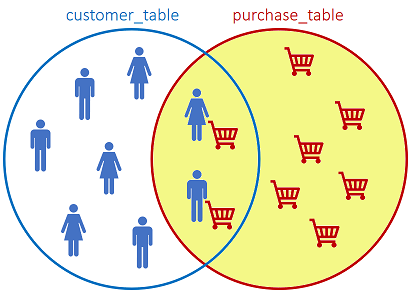
10.3 RIGHT JOIN
The RIGHT JOIN returns all records from the right table, and the matched records from the left table:
SQL statement:
SELECT *
FROM customer_table as customer
 RIGHT JOIN purchase_table as purchase
   ON customer.id = purchase.customer_id;
Output:
 id | age | gender | purchase_id | product_id | price  | customer_id
----+-----+--------+-------------+------------+--------+------------
  1 |  27 | Female |           1 | SX145      |  59.99 |           1
  2 |  27 | Female |           2 | DE438      |  19.99 |           2
  4 |  18 | Male   |           3 | TG671      |  39.99 |           4
  5 |  23 | Male   |           5 | PO876      | 200.00 |           5
  7 |  28 | Female |           9 | CV761      | 120.00 |           7
  8 |  27 | Male   |           4 | ZR565      | 129.99 |           8
  8 |  27 | Male   |           7 | VF455      |  69.99 |           8
  8 |  27 | Male   |           8 | WS130      |  75.00 |           8
 12 |  32 | Female |           6 | LI657      |  25.50 |          12
(9 rows)
In Python:
pd.merge(customer_table,
         purchase_table,
         left_on='id',
         right_on='customer_id',
         how='right')
In R:
customer_table
    %>% right_join(purchase_table, by=c('id' = 'customer_id'))
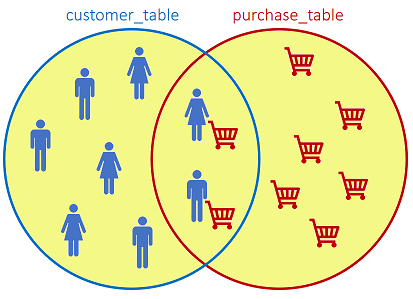
10.4 FULL JOIN
The FULL JOIN returns all records when there is a match in either left or right table:
SQL statement:
SELECT *
FROM customer_table as customer
  FULL JOIN purchase_table as purchase
    ON customer.id = purchase.customer_id;
Output:
id  | age | gender | purchase_id | product_id | price  | customer_id
----+-----+--------+-------------+------------+--------+------------
  1 |  27 | Female |           1 | SX145      |  59.99 |           1
  2 |  27 | Female |           2 | DE438      |  19.99 |           2
  3 |  45 | Female |             |            |        |
  4 |  18 | Male   |           3 | TG671      |  39.99 |           4
  5 |  23 | Male   |           5 | PO876      | 200.00 |           5
  6 |  43 | Female |             |            |        |
  7 |  28 | Female |           9 | CV761      | 120.00 |           7
  8 |  27 | Male   |           4 | ZR565      | 129.99 |           8
  8 |  27 | Male   |           7 | VF455      |  69.99 |           8
  8 |  27 | Male   |           8 | WS130      |  75.00 |           8
  9 |  19 | Male   |             |            |        |
 10 |  21 | Male   |             |            |        |
 11 |  24 | Male   |             |            |        |
 12 |  32 | Female |           6 | LI657      |  25.50 |          12
 13 |  23 | Male   |             |            |        |
(15 rows)
Python:
pd.merge(customer_table,
         purchase_table,
         left_on='id',
         right_on='customer_id',
         how='outer')
R:
customer_table  %>%
    full_join(purchase_table, by=c('id' = 'customer_id'))
Remarks:
- There are minor differences in how the JOIN operation is performed between relational database systems and R.
For example, in the way databases and R treat NA/NaN values: dplyr join functions²⁸ treat two NA or NaN values as equal, while databases don’t.
This behaviour can be modified by passing the na_matches argument with a value of never to the dplyr join functions, thus leading to a result more comparable to the database JOIN in regard of NA/NaN treatment. - pandas provides also pandas.DataFrame.join() to perform JOIN operations. Although it is very similar to pandas.DataFrame.merge(), the two methods present differences that are discussed in detail here²⁹.
11. Conclusions
- There are different ways to achieve the same result. In this post, we summarized the most common SQL queries used for data manipulation and, for each one, provided one of many possible counterparts in both Python and R languages. The purpose of this post is to share useful practical examples as well as a mean to appreciate the similarities between Python, R and SQL.
- The SQL queries were written for PostgreSQL, a popular open source relational database management system. Different databases may present slightly different SQL flavours.
- The statements we explored in this post are not in-place, meaning that they do not change the underlying data structure. For example, selecting the distinct rows with customer_table.drop_duplicates() does not delete the duplicate rows from customer_table. In order to persist the change, we should assign the result, e.g.: new_dataframe = customer_table.drop_duplicates(). This applies to R and SQL as well. For completeness, we remind that many pandas methods support also in-place operations by acccepting the inplace argument set to True (by default, this parameter is set to False). R also supports in-place operations by modifying the chain operator from %>% to %<>%. Examples follow:
Python:
# not in-place: customer_table is not filtered
customer_table.drop_duplicates()
# in-place: customer_table is filtered
customer_table.drop_duplicates(inplace=True)
R:
# magrittr is the R package that provides the chain operator
library(magrittr)
# not in-place: customer_table is not filtered
customer_table %>%
  filter(gender=='Female')
# in-place: customer_table is filtered
customer_table %<>%
  filter(gender=='Female')
12. References
[1] pandas.pydata.org/docs/index.html
[3] pandas.pydata.org/docs/reference/frame
[4] postgresql.org/docs/10/sql-commands
[5] rdocumentation.org/packages/base/versions/3.6.2/topics/data.frame
[6] pandas.pydata.org/docs/reference/api/pandas.DataFrame.append
[7] rdocumentation.org/packages/tibble/versions/3.1.6/topics/add_row
[8] pandas.pydata.org/docs/reference/api/pandas.DataFrame.head.html
[9] rdocumentation.org/packages/utils/versions/3.6.2/topics/head
[10] pandas.pydata.org/docs/reference/api/pandas.DataFrame.drop_duplicates
[11] dplyr.tidyverse.org/reference/distinct
[12] pandas.pydata.org/docs/reference/api/pandas.DataFrame.iloc
[13] pandas.pydata.org/docs/reference/api/pandas.DataFrame.sort_values
[14] dplyr.tidyverse.org/reference/arrange
[15] pandas.pydata.org/docs/reference/api/pandas.DataFrame.describe
[16] rdocumentation.org/packages/base/versions/3.6.2/topics/summary
[17] pandas.pydata.org/docs/reference/api/pandas.Series.value_counts
[18] pandas.pydata.org/docs/reference/api/pandas.DataFrame.groupby
[19] rdocumentation.org/packages/dplyr/versions/0.7.8/topics/group_by
[20] rdocumentation.org/packages/dplyr/versions/0.7.8/topics/summarise
[21] pandas.pydata.org/docs/reference/api/pandas.DataFrame.replace
[22] dplyr.tidyverse.org/reference/mutate
[23] pandas.pydata.org/docs/reference/api/pandas.DataFrame.apply
[25] pandas.pydata.org/docs/reference/api/pandas.DataFrame.drop
[26] rdocumentation.org/packages/dplyr/versions/0.7.8/topics/select
[27] pandas.pydata.org/docs/reference/api/pandas.DataFrame.merge
[28] dplyr.tidyverse.org/reference/mutate-joins
[29] pandas.pydata.org/pandas-docs/stable/user_guide/merging
Data Manipulation in SQL, Python and R — a comparison was originally published in Towards Data Science on Medium, where people are continuing the conversation by highlighting and responding to this story.
from Towards Data Science - Medium https://ift.tt/3qL3ady
via RiYo Analytics


ليست هناك تعليقات