https://ift.tt/3ylji8W A detective novel on how to address high dimensional data This is the story of the paper “Gradient-based Competitiv...
A detective novel on how to address high dimensional data
This is the story of the paper “Gradient-based Competitive Learning: Theory” by me and my students Pietro Barbiero, Gabriele Ciravegna and Vincenzo Randazzo. If you have nothing better to do, you can download it here.

The background
Recently, I was working in the field of deep clustering. It is interesting to see how I can merge deep learning, which is mainly supervised (CNN, MLP, RNN) with clustering techniques, which have an unsupervised nature. Indeed, their behavior is so different that they do not integrate well. Look at this classical scheme:
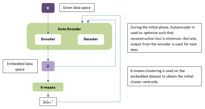
Even if the reconstruction and the clustering loss are often merged, the truth is that the deep learning module is a simple feature extracting and dimension reducing tool for preprocessing of the clustering module. Is this a true integration? Based on this observation, I began studying possible solutions with my team of master and PhD students. But a surprise awaited me …
The mystery
I was working on an interesting application of deep learning to cancer genomics, when, suddenly, I got a strange phone call in the middle of the night. It was Pietro Barbiero, one of my most brilliant students. He was using a very simple competitive layer when he tried to do something very strange. Instead of using the training set data matrix, he tried to use its transpose. This makes no sense! The features become the samples and viceversa. However, the outputs were the prototypes of the clustering! IMPOSSIBLE. Check it better. If this were right, there would be no curse of dimensionality problem anymore. The high dimensionality becomes a larger training set, which results in a positive effect. I could’t believe it.
We spent several days checking this phenomenon, but we always got excellent results. How was that possible? I was struggling to find a logical explanation. It had to be there, even if it was counterintuitive. The results were in front of me. They were absurd, but I couldn’t ignore them. They told me that there had to be an interpretation. But which?
First investigations
So then…
The competitive layer estimates the prototypes through the weight vectors of its neurons, while the output is not very significant. Instead, the same layer, with the same loss function, but with the transposed input, has the significant output (they are the prototypes), while the weights support learning. From this point of view, it can already be said that only this second network is truly neural in nature.
Struggling about this idea, I had the intuition to imagine a principle of duality that binds the two networks. And this is my first result:
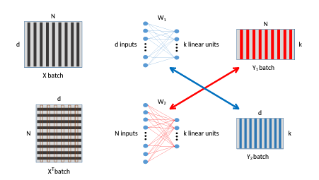
The network at the top represents the vanilla (base) competitive layer (VCL), which is the basis of most clustering neural networks. The vertical lines in the input are the data samples. After training, the weight vectors associated to the output neurons estimate the data prototypes. The bottom network, that I called DCL (Dual Competitive Layer), outputs the prototypes after a batch/minibatch presentation (the rows of the output matrix). The colors in the figure represent the duality (same color = same values). The following theorem resumes my first analysis:
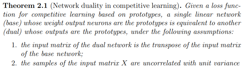
The second assumption is respected by data normalization if the layer is used alone or by batch normalization if it is the final step of a deep neural network for clustering.
About the data topology, we applied the Competitive Hebbian Rule for estimating the edges.
As for training, both networks have to minimize the quantization error, as usual. We added another term to the loss for minimizing the adjacency matrix 2-norm in order to force the sparsity of the edges.
Okay, I had found a principle of duality, but I was far from satisfied. However, a very significant first result, a consequence of this principle, justified the importance of DCL in deep learning. As I told you before, the nature of deep supervised learning and clustering do not integrate well because of their different nature. Indeed, the backpropagation rule, as you can clearly see from a computational graph like this, for RNNs,
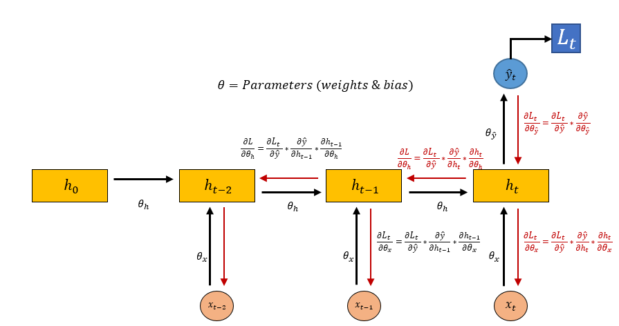
is based on the propagation from the outputs to the inputs of each node, by means of a local gradient. The weight gradient estimation is only a by-product of this propagation. But what if the output is not meaningful, as in deep clustering? Instead, DCL perfectly integrates with the deep modules, as you can see in the following figure, which illustrates the architecture of the deep version of DCL.
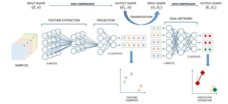
DCL is the only competitive layer that integrates perfectly into a deep neural network (deep DCL).
The mystery deepens more and more
Unfortunately, my students’ experiments on VLC and DCL showed the distinct superiority of DCL. How was that possible? Look at these comparisons on benchmark synthetic datasets.
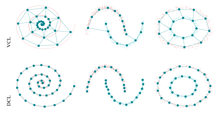
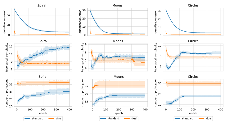
By considering the quantization error, both networks tend to converge to similar local minima in all scenarios, thus validating their theoretical equivalence. Nonetheless, DCL exhibits a much faster rate of convergence. The most significant differences are outlined (i) by the number of valid prototypes, as DCL tends to employ more resources, and (ii) by the topological complexity, as VCL favors more complex solutions. VCL works better. Why? Why? My desperate cry pierces the night. The mystery deepens, and I remain in the darkest anguish. My duality theory was absolutely unsatisfactory in explaining these results. In fact, we weren’t using deep versions, when the best integration had nothing to do with it. I was desperate. I had only two options, either to sabotage my students’ PCs with a virus to worsen the DCL results, or to tackle the problem head on with a new theoretical approach.
It was time to lift the veil from my despair and face the problem with courage. The problem was very simple and I explain it in a very trivial way. Let’s say we have a training set of 4 samples of size 100000. If I could transpose it, as in DCL, I would end up with a dataset of 10000 samples of size 4. Other than curse of dimensionality! Where’s the catch? Well, in the meantime I could already say that the curse of dimensionality reappears when we need to estimate the Voronoi sets of the prototypes, in order to evaluate the quantization error. A sigh of relief! It now had to be seen whether, however, DCL performed better than VCL for high-dimensional data. In a few words, how much does the curse of dimensionality affect DCL? So, I asked my students to check the results of VCL and DCL in version also deep w.r.t. the dimensionality of the problem.
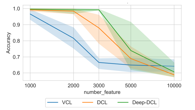
Despite my observation on the problems in estimating the Voronoi sets, it was evident how DCL and, even more so, thanks to its superior integration capabilities, deep DCL give excellent results. In particular, the dual methods yield a close to 100% accuracy until 2000–3000 features! Again, DCL was surprising me.
It was time to use my deductive method to solve the mystery. It was time for math! It might seem like an obvious choice, but let’s not forget that deep learning has seen new techniques flourish often supported solely by empirical explanations. How to say, do you want to be a deep learning expert? Take DCL as it is, thank you, and move on to something else.
A glimpse of light illuminates the darkness
Where to start? The training of both methods is gradient-based, as usual in deep learning. So I decided to follow this path. Let us first analyze the asymptotical behavior of the gradient flow and, then, its dynamics. I must necessarily find an explanation, DCL works, it is undeniable.
First steps towards solving the mystery
At first, I used the stochastic approximation theory for analyzing the asymptotic properties of the gradient flows of the two networks. About VCL, I found the gradient flow is stable and decreases in the same exponential way, as exp(−t), in all directions. This means the algorithm is very rigid, because its steady state behavior does not depend on data. Promising result for me! Much more interestingly, I found the DCL gradient flow depends on data.
In a few words (if you want to see Eq. 34, you are welcome to download my paper), this statement claims the dual gradient flow moves faster in the more relevant directions, i.e. where data vary more. Indeed, the trajectories evolve faster in the directions of more variance in the data. It implies a faster rate of convergence because it is dictated by the data content, as already observed in the numerical experiments, shown above.
Well, I’ve finally elucidated part of the mystery. Now is the time to conclude the investigation. I feel I have the culprit in hand.
The final “coup de theatre”
I did not imagine that the twist was around the corner when I set about studying the dynamics of the two gradient flows. At first I realized that the VCL gradient flow evolves in the range space of its input matrix, while the dual one in the range of its transpose. This fact has very important consequences. For example, the DCL flow is an iterative least squares solution, while the VCL one does the same only implicitly. In the case d > n (being d is the dimension of the input and n the number of samples), which is the most interesting, the VCL gradient flow stays in a space of dimension d, but, asymptotically, tends to lie on an n-dimensional subspace, namely the range of X. Instead, the dual gradient flow is n-dimensional and always evolves in the n-dimensional subspace representing the range of the transpose of X. Consider that both the input matrix and its transpose have the same rank in this case. Look at the following figure, which illustrates this analysis.

Notice that the VCL and DCL solutions are related by a linear transformation represented by the pseudoinverse of X.
I had finally arrived at the solution of the mystery. The culprit was unmasked by the following two theorems.


Above all, the first theorem is the basis of the claim the dual network is a novel and very promising technique for high-dimensional clustering. Indeed, the DCL gradient flow is driven towards the solution remaining in the tunnel of a subspace whose dimensionality does not depend on the dimensionality of the data. Here is the great discovery! However, don’t forget that the underlying theory is only approximated and gives an average behavior.
Epilogue
I have presented to you an important contribution to deep clustering. But, instead of just describing my article, I also wanted to show you the thought process that led me to rationally explain a discovery made by a student of mine. Do not forget, however, that one must never limit oneself to an empirical explanation of the observed phenomena. Stop seeing neural networks as black boxes. Now I am finally at peace with myself, ready for a new investigation. Soon!
The birth of an important discovery in deep clustering was originally published in Towards Data Science on Medium, where people are continuing the conversation by highlighting and responding to this story.
from Towards Data Science - Medium https://ift.tt/3EO0b9Q
via RiYo Analytics


ليست هناك تعليقات