https://ift.tt/3yxELeQ An overview for building interpretable models Karan Taylor Sprezzatura is the art of making something look natu...
An overview for building interpretable models

Sprezzatura is the art of making something look natural and polished. In the picture above, Karan takes care to make a croissant look natural. Similarly, it takes hard work to turn a machine learning model into a handful of rules. Instead, data scientists build complex ensembles of 107 models to win the Netflix recommendation content. We see deep learning models boasting a 100% accuracy, that are riddled with methodological flaws when closely examined.
This post seeks to apply the art of sprezzatura to machine learning. Besides gaining style, your models will be simpler to understand, widely adopted, and easy to deploy.
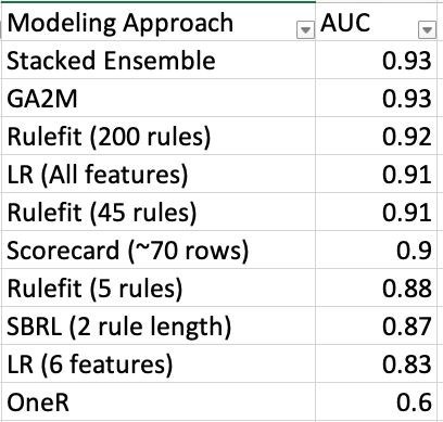
The bulk of this post evaluates four general approaches for interpretable models starting with the most flexible and accurate approaches and moving to the simplest approaches. Some of these are close to the performance of a black box AutoML ensemble model! The approaches include the rulefit algorithm, the GA2M (Generalized Additive Models plus Interactions) algorithm, rule list algorithms, and scorecard approaches. The adult dataset is used as a benchmark. A sneak peak of the final results is shown in this plot.
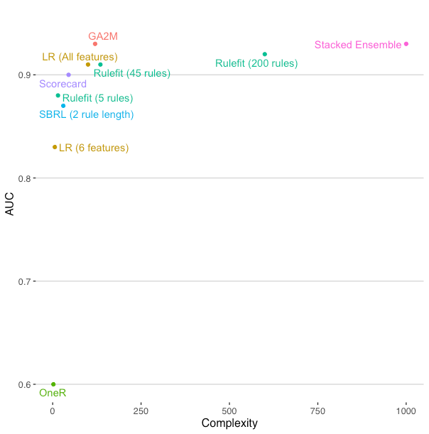
Spoiler alert: two of the interpretable approaches finished equal to or just under the stacked ensemble AutoML model consisting of 20 individual models!
Structure of this post:
- Why use interpretable models
- Building baseline models
- Rulefit algorithm
- GA2M algorithm
- Rule sets models
- Scorecard models
My motivation for this post is as a data scientist who has long cared about model interpretability and explainability. You can also find a video of this talk at the St. Louis Machine Learning and Data Science Meetup. You can also access notebooks with complete code for running these interpretable models are available in the rulez Github.
Why use interpretable models
Interpretable models are unfamiliar to most data scientists. They are defined as a subset of modeling approaches with an emphasis on the sparseness of features and the ability to understand how these features interact with each other to produce a prediction. Consequently, these models are easier to debug and non-technical business stakeholders and regulators alike more readily trust them. An additional, unexpected, benefit is that simpler models are often much easier to operationalize!
Building models involves several steps including problem setup, labeling data, feature engineering, feature selection, algorithm selection, and implementation. This post (and much of the data science literature) focuses on algorithm selection. In reality, building interpretable models and solutions requires all of the steps mentioned here, not just selecting the right algorithm. For example, multicollinearity has a strong effect on model interpretability. So while this post focuses on algorithm selection, let’s call out that model selection is only part of the solution.
Reading academic articles you would think algorithm selection is the main focus of a data scientist's work. This stream of work emphasizes incremental improvements as measured by predictive accuracy. Similarly, Kaggle style model competitions emphasize winning by improved accuracy, however, slight the improvements. While accuracy undoubtedly is important, other concerns like interpretability suffer.
First, the most accurate models are often unusable in an enterprise setting. The winning model of the $1 million Netflix competition was an ensemble of 107 other models. While this model was the best for accuracy, it was simply too complex for Netflix to implement.
Second, these complex models are hard to explain. Practically, this means stakeholders affected by the model don’t trust a model that they don’t understand. Within regulated enterprises, model risk management teams, whose focus is to manage the risk of machine learning models, are resistant to approve complex models. Too many failures can be attributed to black-box models which were later revealed to have simple flaws, such as target leakage. Finally, complex models can be brittle and unusable under conditions of data shifts. Understandable models can be easier to diagnose and modify when data shifts are a concern.
An alternative is starting with an interpretable model. Let’s consider a practical problem and then apply interpretable models.
Problem: Predicting Income
Let’s use the adult dataset from UCI to directly compare complex and simple approaches. This is a public domain dataset used to predict income based on demographic and tax information. The dataset contains over 30,000 observations and contains a mixture of continuous and categorical features. These features have collinearity and interaction effects. The size and complexity are analogous to many tabular datasets within an enterprise setting.
Baseline Models
The first step is building a couple of baseline models. This is an important (and sometimes overlooked) step when modeling. A baseline lets you better understand how much signal you have in a model, what features are important, and how much lift other algorithms provide. All of these are useful data points for helping you understand how much effort you should put into refining your model.
As you start calculating your baselines, you should already have some expectations around the requirements of the final model. Your business partners should help you understand the sort of predictive performance that is needed to bring value to the organization, requirements around deployment, and how stringent the model review process will be.
I am going to start by using three different algorithms for a baseline. Yes, three! They all have different uses and it’s good to use them all. They are the logistic regression, an AutoML stacked ensemble, and an OneR rule-based model.
Logistic Regression
Predicting income with the adult dataset is a classification problem. I would suggest the appropriate starting point for a baseline model is a logistic regression model. The additive nature of a logistic regression is easy to understand and gives us a well-know benchmark for comparing against other algorithms.
For this dataset, I built a logistic regression (LR) model with a few commands using the open source H2O package:
glm_model = H2OGeneralizedLinearEstimator(family= "binomial", lambda_ = 0, compute_p_values = True, remove_collinear_columns = True)
glm_model.train(x, y, training_frame= train, validation_frame=valid)
I built two models, a very simple logistic regression only using the numeric features and a more complex logistic regression using the categorical and numerical features. In this case, adding in the categorical features did noticeably improve the model.
The model results:
- LR (6 numeric features): A logistic regression model with an AUC of 0.83.
- LR (6 numeric & 6 categorical features): One hot encoding of the categorical features led to 100 predictors for a logistic regression model with an AUC of 0.91.
A logistic regression model is generally regarded as easy to understand and widely considered as very interpretable. The coefficients together can be used to calculate a prediction. This transparency is an important reason why LR is well accepted in regulated industries.
The transparency of the logistic regression model often leads people to assume it’s an easily understood model. However, that is not always the case. Adding a large number of features, especially with multicollinearity present, can make understanding a logistic regression model very difficult. Poursabzi-Sangdeh’s research found going from 2 features to 8 features had a measurable impact on the understandability of a model. So while coefficients are helpful, they are not a panacea when the goal is an easily understandable model.
AutoML Stacked Ensemble
AutoML allows us to quickly compare different types of feature engineering and algorithms. I use the H2O’s AutoML to build a challenger.
aml = H2OAutoML(max_models=20, seed=1)
aml.train(x=x, y=y, training_frame=train)
The model results:
- AutoML H2O: The best model was a stacked ensemble of all 20 models with an AUC of 0.93.
This is a highly accurate but complex result. A stacked ensemble of 20 models contains literally tens of thousands of decision points for every prediction. While explanation methods can give you a fairly good understanding of what the model is likely to do, most model risk assessments would fail such an approach. It is simply too complex. Nevertheless, this gives us some idea of the upper bounds of predictive performance.
OneR
OneR builds a model using one feature. It is extremely interpretable and very simple. It is basically a decision tree with only one split. The model works by looking through all the features and selects one feature for the final model. You can find multiple implementations of OneR for R and python.
from imodels import OneRClassifier,
clf = Pipeline(steps=[('preprocessor', preprocessor),
                      ('classifier', OneRClassifier())])
clf.fit(X_train, y_train)
Running this on the adult dataset gives us a simple rule:
If the capital gain is greater than $5,178 then it’s extremely likely that the person is high income.
This model is better than random, but worse than our other baseline models with an AUC of 0.60. OneR is a good check as a baseline and a guard against target leakage. In some cases, you may find enough lift from one feature that deploying a simple rule is more useful than a more complex model.
Summary of Baselines
It should be fairly evident here between the tradeoff of the number of features, the complexity of the models, and the predictive performance.
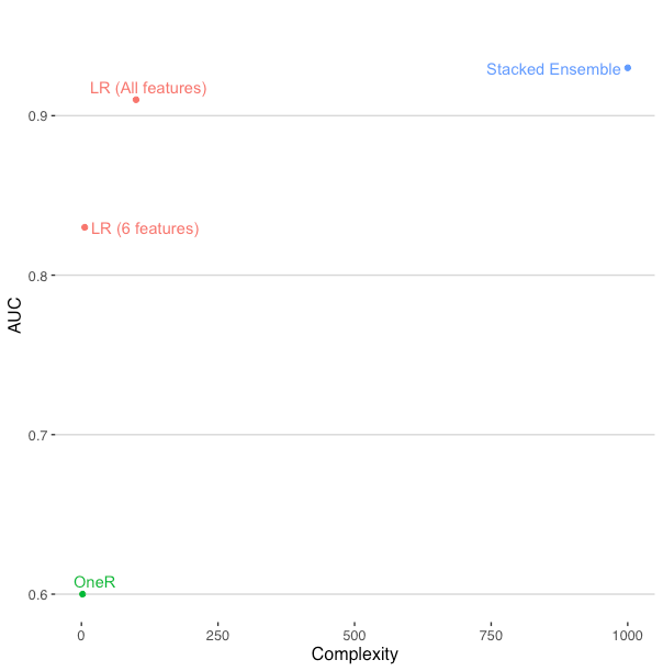
The complexity here is a fabricated number that approximately represents the number of parameters in a model. It is intended to highlight the difference in complexity of the OneR to the stacked AutoML ensemble. This allows us to better understand the tension between improving our predictive performance and the complexity of the resulting model.
The OneR results established that more than one feature is necessary. Running models with just numerical and categorical features separately, it became clear that both numerical and categorical data are providing useful signal. This become important as we think about different ways to represent these features and what model types work best. Finally, we see that complex algorithms and ensembles do add some lift. This suggests some complexity in the data that is not captured in our current set of features. These clues might reflexively push a data scientist to use a sophisticated approach and be done with the problem. However, let’s consider some alternative approaches that will be easier to understand, deploy, and maintain.
Rulefit
The RuleFit algorithm by Friedman and Popescu (2008) is an interpretable model capable of providing high predictive performance along with understandable rules. It’s very easy to use and there are many implementations available. The rulefit algorithm creates an overlapping set of rules.
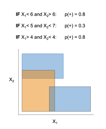
H2O has recently added an implementation of rulefit and it’s quickly become my favorite. Let’s start by building a simple model using 5 rules.
from h2o.estimators import H2ORuleFitEstimator
# Build and train the model:
rfit = H2ORuleFitEstimator(max_num_rules=5,seed=1,
                           model_type='rules')
rfit.train(training_frame=train, x=x, y=y,validation_frame=valid)
Let’s next show you the rules the model created:
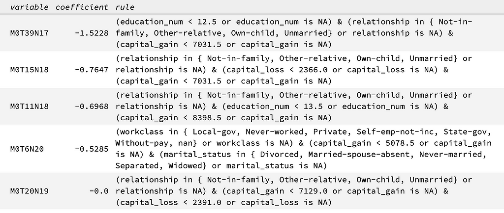
Similar to logistic regression model, for a given prediction you would identify the coefficients/rules associated with the prediction. For example, the top rule applies when when education is less than 13, capital gain is less than $7031, and relationship is Not-in-family, other-relative, own-child, unmarried. This is the strongest rule for predicting someone has low income in the Adult dataset.
The performance of this model is not great. The rulefit with 5 rules gets a 0.80 AUC performance on the test set. The likely issue is that the rulefit is a decision tree approach, which means it creates splits in continuous data. Looking at the rules, you see a mixture of categorical ones, e.g. relationship and continuous ones, e.g. capital gain. With five rules, it’s really hard to capture those continuous features.
A nice bonus feature of the H2O implementation is to combine a linear model with a decision tree for building the rules. This combines the strengths of both models with using linear relationships that constantly change along with decision trees that are effective at binning and interactions. By adding in linear components, here is a rulefit model with 5 rules that achieves a 0.88 AUC.
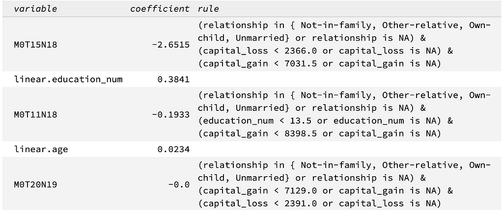
The linear rules are fairly straightforward to understand. For example, as education_num and age increase, so does the probability of a prediction for high income.
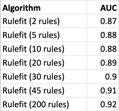
This reinforces that there are strong linear effects for this dataset. The performance jumped from 0.80 to 0.88 by adding linear effects. Any method that relies just on a handful of decision trees is going to be limited in it’s performance. Let’s next vary the number of rules and evaluate how they affect the performance of the model. Here are some results:
To illustrate the flexibility of Rulefit, I plotted a range of models with AUC and complexity. OneR has a complexity of 2 while the LR with 100 predictors has a complexity of 100. For the Rulefit models, complexity was the number of rules multiplied by three (since three features were permitted for every rule).
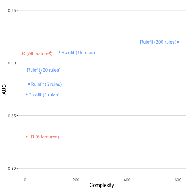
In sum, H2O’s Rulefit offers a lot of flexibility by using both decision trees and linear relationships. Although using lots of rules lets you achieve very high predictive performance, the overlapping rules make it more difficult to understand any individual prediction. This can make it much more complicated to trace a prediction or diagnose an issue with the model. Let’s consider another approach for developing a sparser model that still provides good predictive performance.
GA2M
A generalized additive model (GAM) is an interpretable model that is as transparent as a logistic regression model, but can be more accurate. A GA2M model is a GAM that incorporates an interaction term. The addition of this interaction term generally improves predictive performance.
I learned about the GA2M model when working at DataRobot, which has an excellent implementation. An open-source implementation of GA2M is available in Microsoft’s interpretML package. Let’s explore this with the Adult dataset. Fitting a model is straightforward:
ebm = ExplainableBoostingClassifier(random_state=42)
Looking at the model object with the Adult dataset, you will see the following list of features:
ebm.feature_names
[‘age’, ‘workclass’, ‘fnlwgt’, ‘education’, ‘education_num’, ‘marital_status’, ‘occupation’, ‘relationship’, ‘race’, ‘sex’, ‘capital_gain’, ‘capital_loss’, ‘hours_per_week’, ‘native_country’, ‘relationship x hours_per_week’, ‘age x relationship’, ‘marital_status x hours_per_week’, ‘occupation x hours_per_week’, ‘education_num x occupation’, ‘age x capital_loss’, ‘fnlwgt x education_num’, ‘education x capital_loss’, ‘age x fnlwgt’, ‘occupation x relationship’]
The GA2M creates and then selects a handful of interaction features to use in the model, such as “age x relationship”. This selection is very valuable. I routinely examine the interactions the GA2M is using as a way to understand my dataset. Even if my final model is not going to be a GA2M, it’s still very useful for identifying interactions.
For Adult dataset, these interaction features provide a boost in performance with an AUC of 0.93. This is really good! This is comparable to the stacked ensemble model.
The resulting model is transparent with all the coefficients available. It’s even possible to put together a rating table that lists the coefficient factor for each level of a factor. The InterpretML package also includes visualizations so you can see this for yourself. Here we see the different coefficients for marital_status.
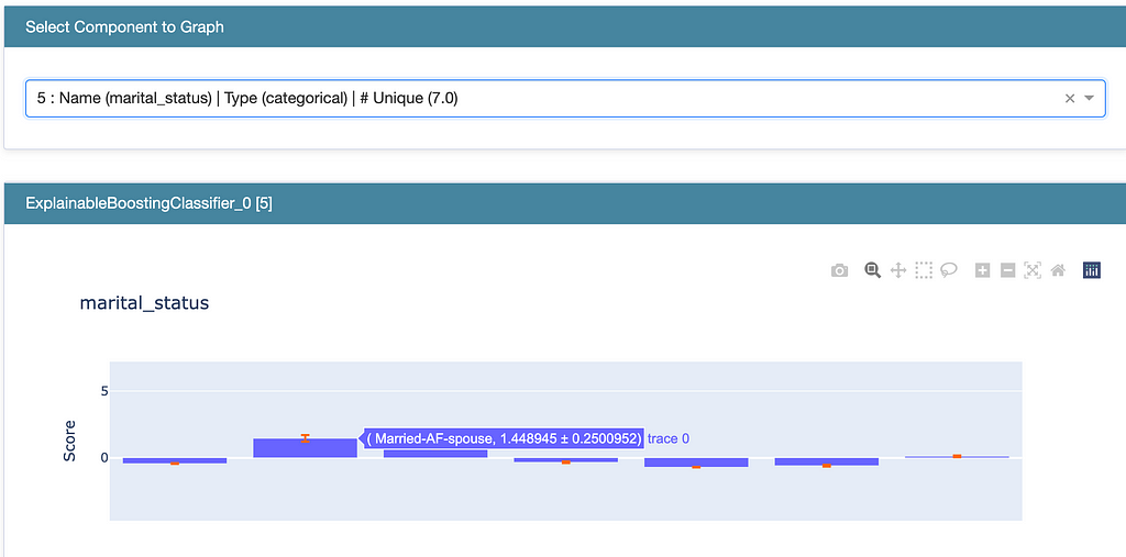
In sum, GA2M models start with the best of linear models, but also mix in the ability to incorporate the best interactions. Finding these interactions is not easy (and you all should use these interactions to inform your own understanding of the problem). By adding these interactions the GA2M often offers very good predictive performance. GA2M’s use of coefficients and a rating table is a well-known practice and well accepted within model risk management practices and regulatory requirements.
Rule Lists
The rulefit algorithm relied on an overlapping rule set. This meant several rules could affect a single prediction. In contrast, rule lists are constrained to not having any overlapping rules. The advantage of non-overlapping rules is that every prediction can be tracked to one rule. This makes the results very understandable.
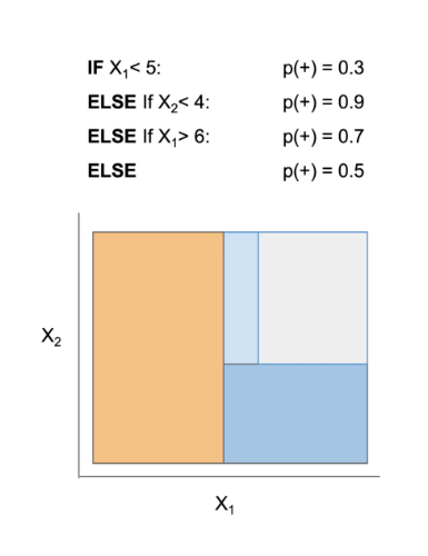
Building rule list models can be computationally expensive. Rule lists also bin continuous features, so linear relationships may be difficult to incorporate into a rule. Finally, current implementations of rule lists are limited to classification problems.
A great starting point for implementations of rule lists is the Interpretable machine-learning models (imodels) package. I started with a well-known approach, Certifiably Optimal RulE ListS (CORELS), but had trouble installing on my Python 3.7+ environment and it was too slow to build anything but a very basic rule list on the Adult dataset.
I found Scalable Bayesian Rule Lists approach worked much faster. This is only available as an outdated R package. My testing is using the adult dataset with its categorical features and a training dataset size of 15,000 rows.
sbrl_model <- sbrl(data_train, iters=30000, pos_sign="1",
                   neg_sign="0", rule_minlen=1, rule_maxlen=1,
                   minsupport_pos=0.003, minsupport_neg=0.003,
                   lambda=10.0, eta=1.0, nchain=10)
print(sbrl_model)
Running this code took just a few seconds using a rule_maxlen=1. Here are the results:
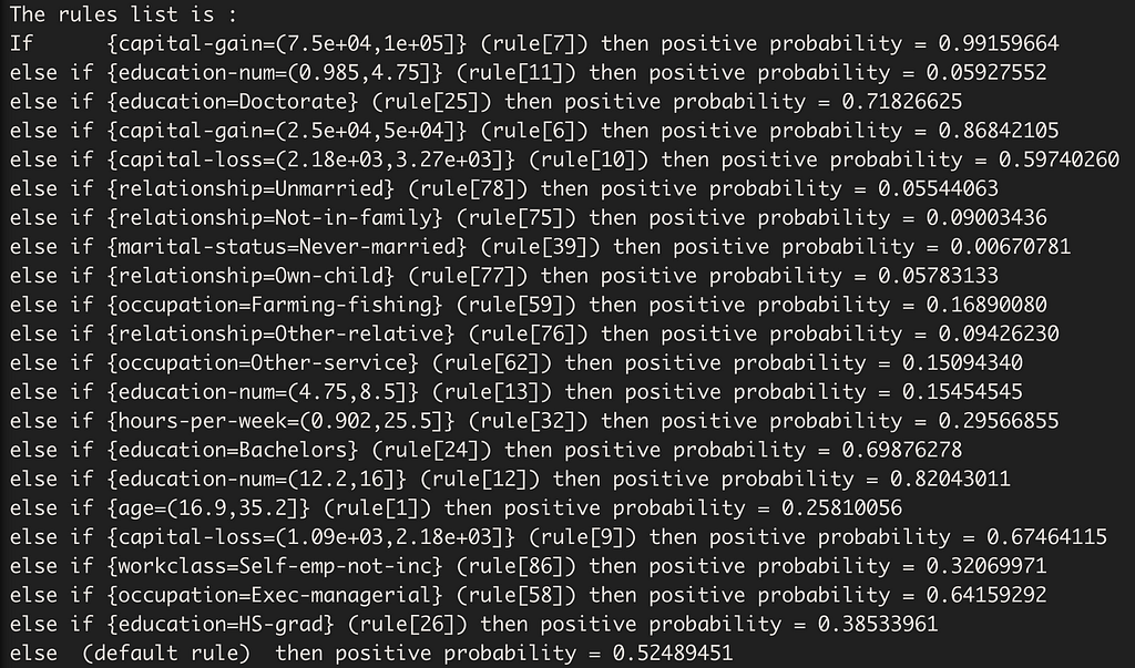
The results are non overlapping rules that are read sequentially. This means anyone could take identify which rule applies to their prediction. It becomes much easier to understand the outcome for any prediction.
The rule list model has a 0.86 AUC, which is a marked improvement from the 0.80 AUC that rulefit found with 5 rules. However, to find this better solution does take extra computation to calculate this best set of rules. It’s possible to improve the performance by increasing the maximum rule length of the SBRL model to 2. This improved performance to 0.87 AUC. This does result in more complicated rules:
if {education-num=(4.75,8.5],marital-status=Married-civ-spouse} then positive probability = 0.14173228
Increasing the maximum rule length increases the search space. Moving to a rule length of 2 took a substantially longer time to calculate. Calculating a rule length of 3 was not possible on my laptop.
The non-overlapping nature of these rules is a huge advantage for interoperability, error detection, and diagnosing issues during deployment. But keep in mind, computing these rules is complex. However, the simplicity of these rules means that often they will lag modern algorithms in predictive performance.
Scorecard
A common interpretable method for decisions is using a scorecard. Scorecards allow for a number of features and the predictive score is based on a simple summation. They are very easy to use and common in fields like health care and criminal justice.
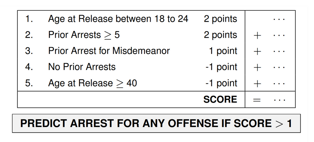
Developing optimal scorecards from machine learning can be computationally challenging. A well-known technique is using Supersparse Linear Integer Models (SLIM). For this post, I used the scorecard function in the OptBinning package. The scorecard point ranges goes from 0 for the lowest probability of income up to 100 for the highest income.
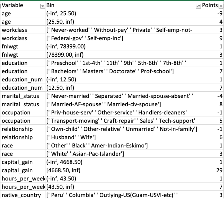
The fairly simple scorecard resulted in an AUC of 0.89. This model is very close to the logistic regression using all the features (100 predictors). However, the scorecard is much easier to explain and deploy than logistic regression coefficients. If explainability is very important, a scorecard approach works very well.
Next Steps
To provide a big picture view, here are the results and a plot of the predictive performance versus complexity. It’s important to understand that each of the techniques, rulefit, GA2M, rule lists, and scorecards, have their distinct tradeoffs. I have shared code at the rulez github repo so you can try them all and choose accordingly.
My hope is this post adds a bit of sprezzatura to your machine learning. Take time to understand your problem, work with your data, and see if it’s good fit for a simpler interpretable model.
There is a much wider universe of interpretable models than is presented in this post. There are other popular interpretable models such as Bayesian methods that provide uncertainties with their predictions. A great starting place, moving beyond Molnar’s interpretability treatise, is Chandan’s imodels package that contains a sampling of many different approaches.
I received great feedback from a number of people, including Jonathan Dahlberg, Taylor Larkin, Chandan Singh, Miles Adkins, Dave Heinicke, and Nishant Gandhi. So a big thank you to all of them.
You can also follow me on Twitter or LinkedIn and find older blog posts on my projects site.
The Art of Sprezzatura for Machine Learning was originally published in Towards Data Science on Medium, where people are continuing the conversation by highlighting and responding to this story.
from Towards Data Science - Medium https://ift.tt/3H5mEAb
via RiYo Analytics

No comments