https://ift.tt/3DKkZh4 Topic modeling, sentiment analysis, and readers clustering to derive insights on users preferences and perform tailo...
Topic modeling, sentiment analysis, and readers clustering to derive insights on users preferences and perform tailored recommendations

Introduction
This posts describes, along with Python code, an analysis of the readers’ comments open dataset from Rome’s libraries made publicly available by “Istituzione Biblioteche di Roma”¹.
The analysis leverages topic modeling techniques to find recurring topics among readers’ comments, and thus determine, by inference, the themes of the borrowed books and the interests of the readers. Moreover, sentiment analysis is performed to determine whether customers comments are positive or negative. Finally, readers data (age and occupation) are used to achieve customers segmentation via clustering techniques.
This provides insights on the topics of borrowed books, the readers sentiment and different readers clusters. On top of that, these information will be used to perform recommendations in two different scenarios:
- Recommendation by topic:
1.1. Find the book titles in the most similar topic
1.2. Return the book titles ordered by descending comment sentiment score - Recommendation by user (when we do not have a preferred topic, but still have some information about the reader):
2.1. Perform clustering on readers’ data (age and occupation)
2.2. Find the belonging cluster for a new user
2.3. Return the book titles ordered by descending comment sentiment score.
Data Preparation and Exploratory Data Analysis
We start by importing the required libraries:
Then we load the dataset¹ (updated at November 2021):
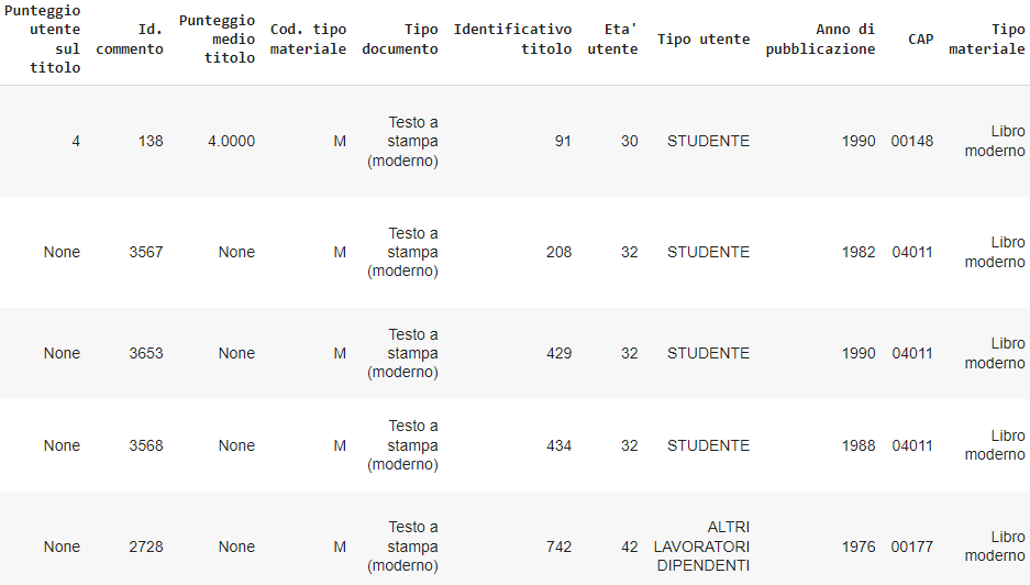
We are mainly interested in the following columns:
- “Descrizione commento”: full user’s review that will be used for topic modeling and sentiment analysis.
- “Titolo”: title of the material (book, movie, ..) borrowed by the customer, and subject of the review.
- “Età utente”: customer’s age in years.
- “Tipo utente”: customer’s occupation.
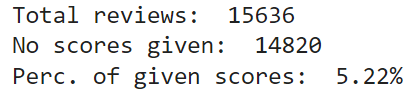
Notably, a column from the dataset collects a score given by the user to the product, from 1 to 5. Nevertheless, out of the 15636 total reviews, only 5.2% display this score, therefore this information will not be used:
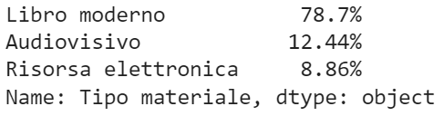
The products being reviewed are books for 78.7%, audiovisuals (such as movies) for 12.44%, and electronic resources for 8.86%:
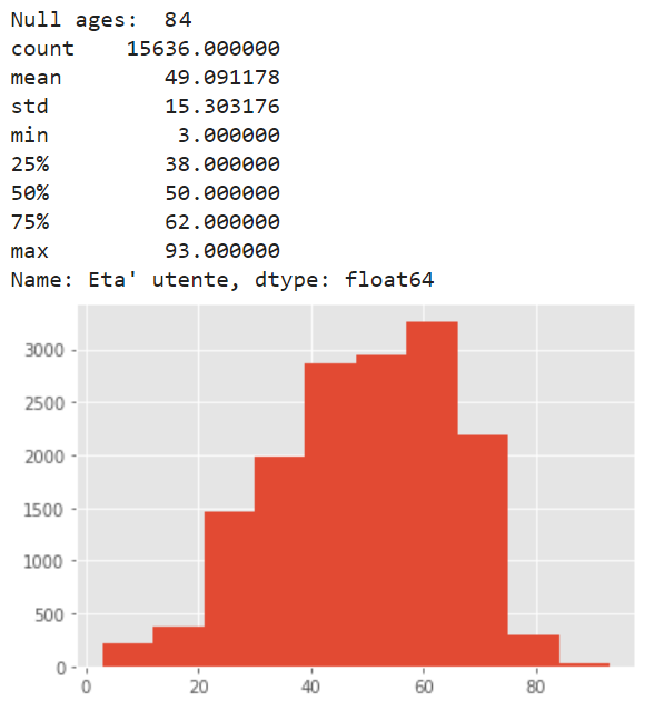
By observing the customers, we notice that they have a mean age of 49 years, (only 25% of overall reviews were written by readers under 38 years), and that there are few missing values:
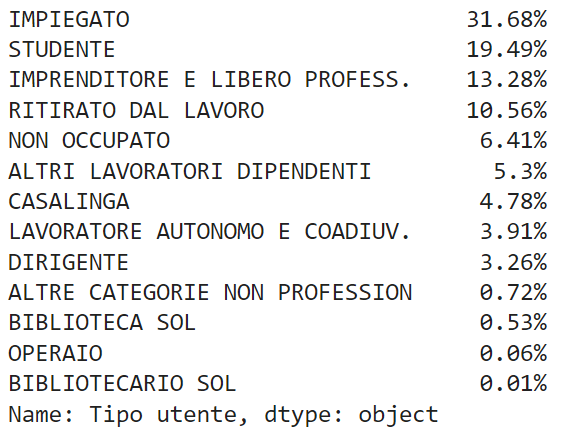
Most of the customers have an occupation, with the most recurrent type of employee (“impiegato”, 31.58%), while students (“studente”) represent only 19.49% of the customer base:
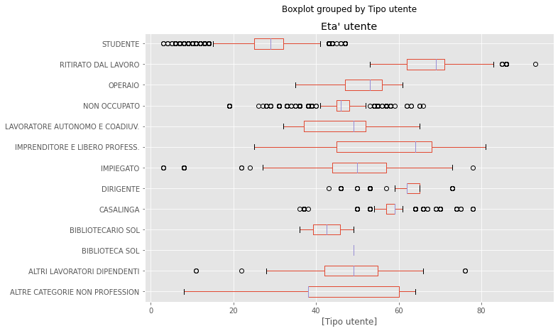
From the distributions of ages by occupation type, we may also observe how students have lower age (mean±std: 26±8, q1–q3: 25-32), than employees (mean±std: 51±8, q1–q3: 44–57) or workers (mean±std: 50±9, q1–q3: 47–56), and retirees (mean±std: 68±5, q1–q3: 62–71).
Topic Modeling
The readers reviews are not associated with any label, therefore they need to be analyzed with an unsupervised approach.
In order to find semantically similar structures among the comments, we are going to use BERTopic², a topic modeling technique by Maarten Grootendorst³.
As explained by the author⁴, the main steps of the algorithm involve the documents embedding, leveraging, among others, BERT⁵; then UMAP⁶ to lower the embedding dimensionality that would otherwise lead to poor clustering performances; HDBSCAN⁷ for clustering, and, finally, the definition of a topic representation by applying the TF-IDF on all documents within the topic (instead of applying it to single documents), basically treating the topic as a document itself (hence the name, class-based TF-IDF): in this way the resulting important words (and related scores) provide a meaningful, interpretable topic description.
We now observe the 25 most recurrent topics in the readers reviews. The topic names are made of the most representative words by the class-based TF-IDF scores, and by looking at their frequency we can derive insights on what customers read:
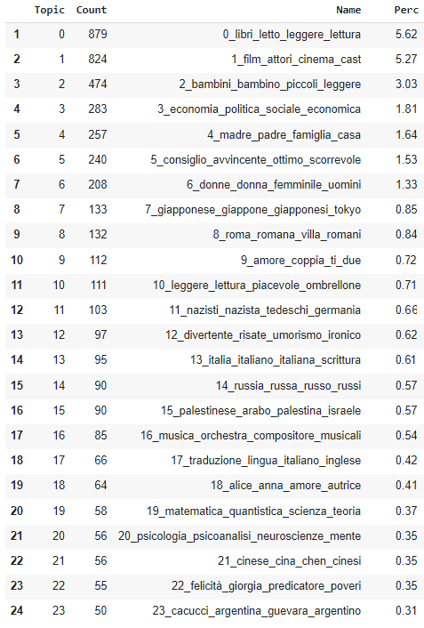
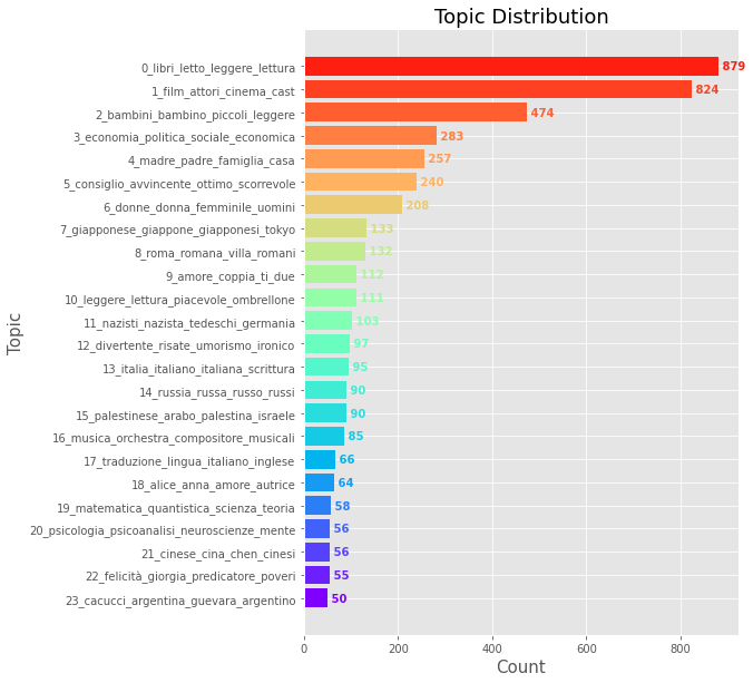
For example, if we observe the table from the top we notice that 5.27% of all reviews are related to movies (topic 1), followed by a 3% of reviews related to children books (topic 2) and a 1.8% of reviews related to socio-economics readings (topic 3).
We may also infer trends or preferences concerning foreign literature or countries, where Japan is object of 0.85% (topic 7) of all reviews, and Russia of 0.57% (topic 14).
We can also see a significant number of reviews (0.84%, topic 8) concerning Roman history and architecture. Perhaps, this may be related to the locality of our observations (readers’ comments from the libraries of Rome).
The question may arise about the reason behind the low fraction of reviews covered by the most recurrent topics. Intuitively, we may expect the most recurring topics to explain the majority of reviews (Pareto principle). There are at least two main reasons for this finding:
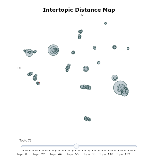
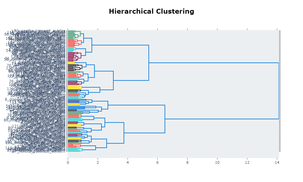
- The sizeable amount of detected topics: repeated experiments on the dataset always led to a consistent number of topics, varying between 130 and 145. In case this high sensitivity to semantic differences produced a result too fragmented to be easiliy interpreted, the number of topics may be reduced. There are different approaches to topic reduction. We can observe topic similarity by their hierarchical structure, and how they relate to one another, for example through topic_model.visualize_topic():
- The presence of outliers: HDBSCAN, the clustering algorithm used in BERTopic, does not force observations into clusters, leading to outliers that are collected in the topic index -1.
We finally save the topics to a new dataframe column:
Sentiment Analysis
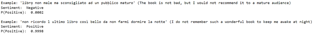
We perform sentiment analysis over the readers reviews to determine whether a comment is positive or negative by using the feel-it-italian-sentiment⁸ model, available on HuggingFace⁹.
The model fine-tuned the UmBERTo¹⁰ model on a new dataset: FEEL-IT, a novel benchmark corpus of Italian Twitter posts.
We can test the model output on few sentences:
And predict the sentiment of comments. This is saved in a new dataframe column:
Notably, we limit the number of words to take under consideration for the sentiment analysis for each comment through the max_w variable.
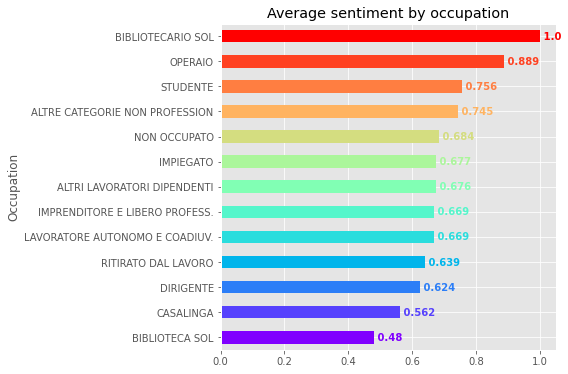
We can also observe the average sentiment by readers occupation, verifying that workers (age: 50±9) and students (age: 26±8) express the most positive sentiment, while housewives (age: 57±6), executives (age: 62±3) and retirees (age: 68±5) manifest the least positive sentiment in products reviews:
Readers’ Clustering
So far, we carried out topic modeling and sentiment analysis on readers comments by exploiting Natural Language Processing techniques.
We now perform customers’ clustering based on their characteristics (age and occupation) in order to later implement recommendations in absence of preferred topics or interests.
As the observations contain both numerical (age) and categorical (occupation) variables, we will use the k-prototypes algorithm¹¹.
Note: as we impute the missing age values by replacing them with their average, we do not perform further preprocessing (age is the only numerical variable we are using), but we might also scale it or apply transformations to make it more Gaussian-like, such as the Yeo-Johnson transformation¹².
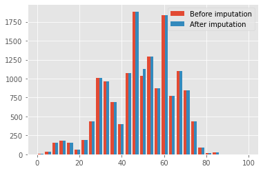
We check whether the age is normally distributed through the Shapiro test:
We use the elbow method to determine the number of clusters:
We fit the model with 4 clusters, from the observation of the elbow on the plot, and then save the information in a new dataframe column:
We can now inspect the obtained clusters, by observing the age distribution and the most recurrent occupations within each cluster:
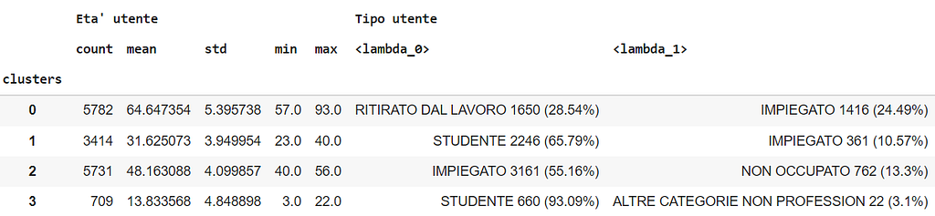
We can summarize the clusters as follows:
- n°0: retired over 60: age between 64.6±5.4 years, most recurrent occupations “retiree” (28.5%) and “employee” (24.5%).
- n°1: students and employees in their thirties: age between 31.6±3.9 years, most recurrent occupations “student” (65.8%) and “employee” (10.6%).
- n°2: workers in their fourties/fifties: age between 48.2±4 years, most recurrent occupations “employee” (55.2%) and “unoccupied” (13.3%).
- n°3: young students: age between 13.8±4.9 years, most recurrent occupation “student” (93.1%).
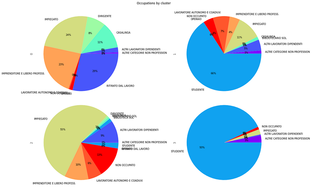
The distribution of occupations by cluster can also be visually inspected:
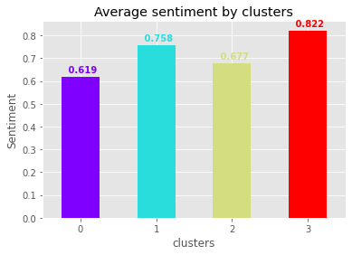
Young students (cluster n°3) manifest the most positive sentiment in reviews (0.82±0.37), while retirees or emplooyees over 60 (cluster n°0) exhibit the least positive sentiment (0.62±0.4):
Recommendations
Recommendation by topic
Let us consider a customer asking a librarian:
Could you recommend something about travels?
Or let us imagine the same customer performing a similar query on an online library catalogue.
Thanks to topic modeling performed on customers reviews, we may find the most similar topic associated to the argument of interest and then, among that topic, recommend the most positively reviewed titles.
Therefore, we define a Recommendation class that takes the topic model and a search query as input, and provides methods to:
- determine the most similar topic,
- display its representation (class-based TF-IDF words scores) through a wordcloud chart, and
- recommend the first n titles based on topic similarity and sentiment score:
Example n°1: vacanza (vacation)
What will be recommended for when searching for vacation (“vacanza”)?

The closest topic has id 53 and a similarity of 0.83, we can observe the topic representation (class-based TF-IDF words scores) as validation of the similarity measure:
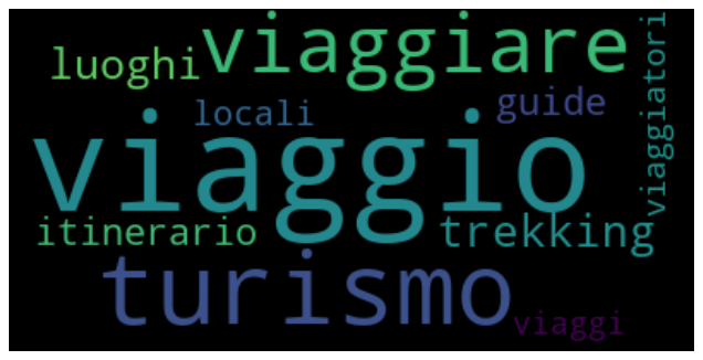
The closest topic to “vacation” is represented by words such as “travels”, “guides”, “tourism”, “itinerary”, “travelers”, “trekking”.
The top 5 titles in that topic by sentiment score are:
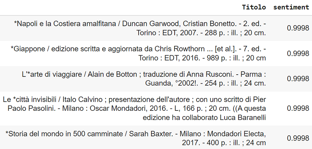
The titles include travel guides (specifically, for Naples, the Amalfi Coast, and Japan), suggesting gateway destinations for the vacation, as well as novels that delve into the concept of travel (Alain de Botton’s “The Art of Travel”, Italo Calvino’s “Invisible cities”).
Example n°2: giallo (yellow/crime fiction)
“Giallo” is an interesting query term: in Italian, such word stands for both the color yellow and the genre of crime fiction narratives.
Steps:
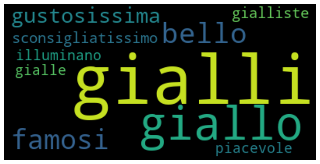
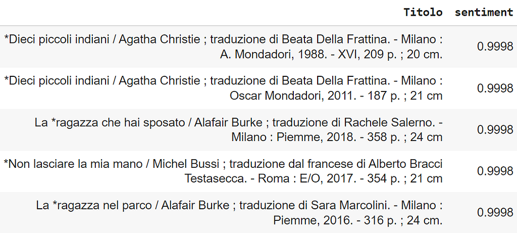
Despite the input word’s ambiguity, all results belong to the crime fiction genre.
Unsurprisingly, Agatha Christie’s “And Then There Were None” shows up as top recommendation for this topic (in two different editions).
Example n°3: jazz
Code is not repeated for simplicity (the same steps from the previous examples can be applied):
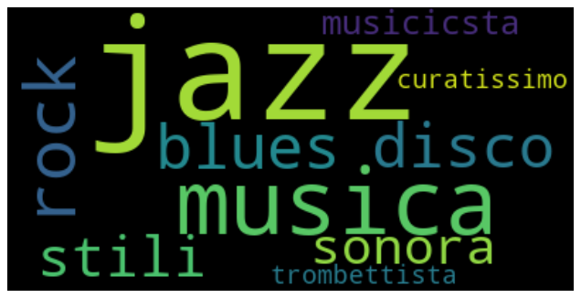
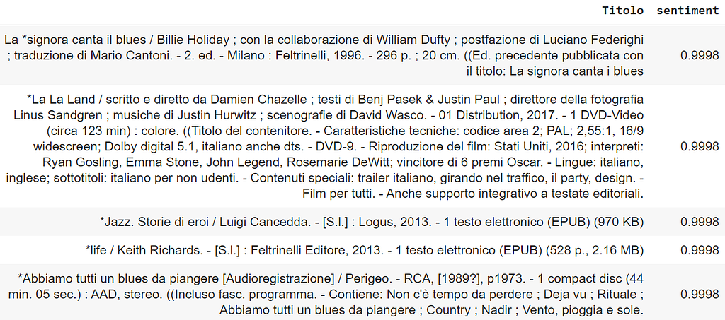
Although I personally find all recommended results interesting, I would like to draw attention to the fifth result: “Abbiamo tutti un blues da piangere”, a marvelous album from Perigeo, a Jazz/Prog Rock italian formation from the 70s, whose existence I was unaware until now. I am sincerely grateful to have discovered this hidden gem (indeed, recommendations seem to work).
Notably, different product types are retrieved (books, movies, albums). This behaviour may be modified by taking into account the product type, either in the modeling phase or in the recommendation phase (e.g. as a filter).
Recommendation by customers characteristics
In a scenario in which a user has no preferred topics or specific interests, and no search/loan history is available, recommendations may be still achieved by exploiting the customer segments produced by clustering.
Given a user’s age and occupation, we could find its cluster of belonging, and return the most positively reviewed titles in that cluster as recommendations:
Let us assume we need to provide recommendations to a 32 years old employee:

As we would expect, the user belongs to cluster n°1, whose elements are students and employees in their thirties. We can now retrieve the most positively reviewed titles in the same cluster:
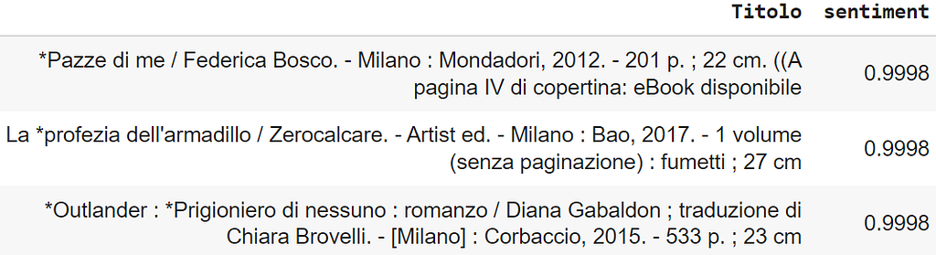
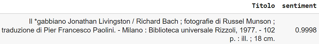
What would be recommended to a 12 years old student?
Conclusions
We analyzed the Rome’s libraries comments dataset, owned and made publicly available by “Istituzione Biblioteche di Roma”.
Topic modeling and sentiment analysis allowed us to derive insights on libraries loans and users’ preferences. Clustering techniques provided additional information over the customer base.
We used these insights to implement a recommendation strategy by employing either topic and sentiment information (“Could you suggest something about travels?”), or, in absence of a query or expression of interest, the customers clusters and sentiment (most positively reviewed titles in the cluster the user belongs to).
Improvements could be made by taking into account the different products natures (books, movies, albums) as filters, and combining the topic of interest with customer segmentation. The number of topics may be also subject of further tuning, although the showed most recurrent topics were consistently identified in different experiments.
References
[1] https://www.bibliotechediroma.it/it/open-data-commenti-lettori
[2]https://maartengr.github.io/BERTopic/index.html
[3] https://medium.com/@maartengrootendorst
[4] https://towardsdatascience.com/topic-modeling-with-bert-779f7db187e6
[5] Jacob Devlin, Ming-Wei Chang, Kenton Lee, Kristina Toutanova, “BERT: Pre-training of Deep Bidirectional Transformers for Language Understanding”, 2019, arXiv:1810.04805v2
[6] Leland McInnes, John Healy, James Melville, “UMAP: Uniform Manifold Approximation and Projection for Dimension Reduction”, 2020, arXiv:1802.03426v3
[7] Claudia Malzer, Marcus Baum, “A Hybrid Approach To Hierarchical Density-based Cluster Selection”, 2020, arXiv:1911.02282v4
[8] Federico Bianchi, Debora Nozza, Dirk Hovy, “FEEL-IT: Emotion and Sentiment Classification for the Italian Language”, 2021, Proceedings of the 11th Workshop on Computational Approaches to Subjectivity, Sentiment and Social Media Analysis, p.76–83 (link)
[9] https://huggingface.co/MilaNLProc/feel-it-italian-sentiment
[10] https://huggingface.co/Musixmatch/umberto-commoncrawl-cased-v1
[11] Zhexue Huang, “Clustering large data sets with mixed numeric and categorical values”, 1997, In The First Pacific-Asia Conference on Knowledge Discovery and Data Mining, p.21–34 (link)
[12] Sanford Weisberg, “Yeo-Johnson Power Transformations”, 2001 (link)
Rome’s Libraries Readers’ Comments Analysis with Deep Learning was originally published in Towards Data Science on Medium, where people are continuing the conversation by highlighting and responding to this story.
from Towards Data Science - Medium https://ift.tt/3IyU1g1
via RiYo Analytics


No comments