https://ift.tt/3za08TJ Experimentation is easy, right? This article links common pitfalls in experiment design with fundamental statistical...
Experimentation is easy, right? This article links common pitfalls in experiment design with fundamental statistical assumptions behind t-tests.
Imagine you split a small portion of your user base into two groups. One group is treated to a new feature, the other one isn’t. You observe that the average revenue of a user in the variant group is higher, and it seems statistically significant: so the feature is good, let’s roll it out! Voila, experimentation is easy. Well maybe…

Experimentation should be easy, by the way: it is the cheat-code for robust causal inference. But if it is done without due care and attention, the wrong conclusions can be made. Spending a bit of time to make your experiments robust can be the difference between making the right or wrong decision for your company.
Here are some top tips behind experimentation, tying it back to first principles to help ensure your conclusions are robust.
Evaluate your experiment design against first principles
In our experiment, we collect small samples that we hope reflect the two parallel universes that we want to compare (say one where a feature is introduced, and another where it isn’t). Hence, the aim of experiment design is to isolate the differences between the test and control group down to just two things:
- The genuine difference in the metric due to your new feature X
- Sampling error (because we only collect a small sample: we will discuss this shortly)
Experiments often use a t-test. A t-test estimates the probability that the mean of the variant group might have come from the same sampling distribution as the mean of the control group. In other words, we are testing the null hypothesis that there is no difference between the control and the variant mean (and even if there is some difference, it is just due to noise in collection).
If testing the difference in a mean metric between a test and control group, and there are more than 30 samples in each, then Welch’s t-test is likely your test of choice.
Ensuring the assumptions behind the Welch test are met will help isolate any measured difference between the groups down to just these two factors. There are two key assumptions to look for when collecting your samples to achieve this:
- Independence of sampling between groups
- Independence and identical distribution (iid) of sampling within groups

So what is independence between groups, and why should I care?
Network effects
Violating independence between two groups could mean the outcome from one group impacts the other group too. Take a social media platform example: you release a new sharing feature to the users in your variant group, and the control group can’t see it. The users in your variant group use the new sharing feature, and more frequently than they used the old one. This increases their mean engagement metric (so looks good so far!). But the users in your control group can’t see these new shares, in fact they now see less than before, so that in turn means they interact with less content than they otherwise would. This decreases their mean engagement metric: the difference between the groups is over-exaggerated. This is an example of a network effect that violates the independence assumption. Similarly, assigning samples to groups at the user level, rather than the visit level, can ensure there is no cross-pollution of effects between groups if the user can see both versions.
Observable confounding factors
A confounding variable is a factor that impacts the assignment of samples to test or control groups, as well as the metric of interest. So violating independence could mean the samples collected might not be equally influenced by the same underlying factors. For example, we run an experiment for a new colour theme for your site, measuring new user sign-up rates: the control group samples are collected on Monday to Wednesday, and the variant samples were collected Thursday to Saturday. But users are more likely to join at the weekend, so all things being equal we would have expected the number of users to be larger on Saturday anyway. The allocation of users to each group is not independent with respect to day of week. Running the experiment at the same time helps solve this, so that’s an easy fix….
Hidden confounding factors!
But now let’s say, coincidentally, there are more colour-blind people in your variant group: this is a factor that impacts your metric, but you don’t collect data on it — so how do you prevent this from confounding your measurement? Randomization is your friend here. Randomly allocating your user base into test and control groups (with a sufficient sample size) tends to balance across even the features you don’t collect data for. It also helps ensure your sample is representative of your population too. To be exact, randomization will not guarantee an equal distribution between the groups, just tend towards it: but the chance of an unequal distribution should be factored into the p-value when testing anyway.
So what is i.i.d within groups, and why should I care?
Check the stationarity of the metric
Independence ensures that the collection of one sample doesn’t impact the collection of another. Identical distribution also implies that the distribution the samples are collected from adequately models the population we hope it represents. In other words, it implies that there are no underlying trends impacting the samples we observe: if the collection of samples impacts the population, then there is no “true” value (it changes as the samples are collected). Instead we should expect the metric to tend towards the true mean as its collected (by the law of large numbers) rather than trend upwards or downwards, or its variance to change over time (which would mean the metric isn’t stationary). However, ‘outside knowledge’ of the data is likely necessary to decide if the data is i.i.d.
But why does this help?
If the assumptions of independence and identical distribution are met, then (assuming a sufficiently large sample size) we can be confident that the means of each sample follow a normal distribution: with a mean tending towards the population mean, and a variance related to the size of the sample. This is the most common version of central limit theorem (CLT) in a nutshell.

To illustrate this: imagine flipping a fair coin. Each coin flip doesn’t impact the next one (independence) and using the same coin ensures the probability of a head remains the same (identical distribution). If you flip the coin 10 times, and record the number of heads, you might expect to get 5. But actually, there is only a ~25% chance you will get 5! This is sampling error: despite the true probability being 50%, you are more likely to not get 5 heads when only flipping it 10 times. For example, there is ~38% chance you get four or less.
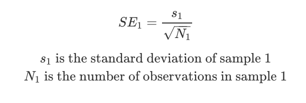
Now imagine an enthusiastic coin-flipper repeated the test — but they did it 100 times. Now the probability that they observe 40 heads is only ~3%. Contrast that to when we only did 10 flips, observing 4 flips or less was 38%! This shows how the more samples we take, the more confident we can be in the results. The standard error is a measure of the standard deviation of these means, and decreases as more samples are collected:
Now imagine a completely eccentric coin-flipper repeated the 100-flip experiments thousands of times, recording the average number of heads each time. Not only would they find the average number of heads per procedure would be 50, but the distribution of these procedure means would follow a normal distribution, with ~68% (one standard deviation of these mean) of the procedures having 45–55 heads and ~95% (two standard deviations) of the procedures having 40–60 heads. CLT means that even though the underlying distribution of coin flips is binomial (observing a head is binary, zero or one) the distribution of the mean number of heads is normal.
Because CLT ensures the distribution of means is normal, meaning we can estimate the sampling error variance (the standard error), we can start to determine the likelihood that the mean we observed in the variant sample was generated from the same distribution as the control. If this probability is low enough, we determine there is a statistically significant difference between the two groups. Thinking critically about whether the assumptions of independence and identical distribution are met thus helps ensure the conclusions from these tests are robust.
FYI — these eccentric experimenters are ‘frequentist’ statisticians. Repeating the procedure many, many times, will give you the correct answer in the long-run (side-note: this is also the correct way to think about confidence intervals: they do not relate to the probability, as either the true mean falls in the estimated confidence interval or it doesn’t; but if you repeat the collection of samples and ‘confidence interval estimation’ procedure many many times, 95% of those CIs will contain the true value).

One extra thing to note: as part of the test, we need to estimate the true mean and standard deviation of our population mean from the smaller samples we collect. This is also only valid if the underlying samples collected are independent and identically distributed (with large enough sample size).
Tying this together: statistical power
The statistical power of the test is the probability we detect a statistically significant difference between the two groups, given there is a genuine difference.
Imagine we have two coins, and we want to determine if there is a difference in their probability of flipping heads. So we flip each one 100 times. From these samples, we estimate the means of the true population as X1 and X2. We estimate the standard error (the standard deviation of these means) as the standard deviation of the sample divided by the square root of the sample size.
In this case, a Welch t-test statistic is specified in the following way:
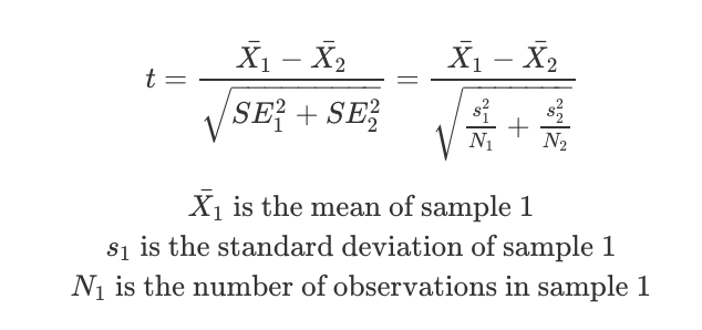
The larger the absolute value of the test statistic, the more likely the result is statistically significant. This implies we are more likely to detect a true difference between the variant and control groups if:
- The difference in the means (X1 — X2) is larger
- The sample size is larger (so N_i is larger)
- The variance of the metric (the noise, s_i) is lower
This illustrates the importance of good metric selection. If the chosen metric is fast-twitch and less noisy, the difference will be larger and the variance lower: hence the absolute t-stat will be larger for the same sample size. We will discuss this shortly.

(Side note: I would always run a Welch t-test rather than a student test: if the population variances are the same, it almost equates to a student t-test anyway)
Some further tips on running effective experiments
Be hypothesis led.
Data scientists are often given a fuzzy question, such as “should we release feature X?”. The first step is to convert this into a testable problem statement that either has a true or false answer. For example, “Feature X will increase the mean number of engagements per user.” The t-test statistic is a good candidate for comparing the difference in group means. Being hypothesis-led ensures your testing is intentional, focused on answering the ‘why’, and is also the backbone behind designing an effective metric.

Spend time designing a few great metrics.
Designing a great metric is often the secret sauce that makes experimentation effective — so intentionally spend time evaluating your metrics. Most importantly, the metric you design has to be highly correlated with the goal your company cares about. But on the flip-side, often these company-level numbers are just too slow-moving: increasing revenue or the number of users on the platform is an admirable goal, but it’s really unlikely you’re going to be able to move it meaningfully during your small experiment. Instead, focus on ‘fast-twitch’ metrics, such as those measuring conversion rates or user engagement: this might be a difference between the two groups you can meaningfully measure (and that you know in the long-run is correlated with driving more revenue or more users).
It is also worth spending time to think about the pitfalls of your metric, so that it can’t be ‘gamed’. For example, you could run a misleading advertising campaign that increases click-through rates, but that will be a bad experience for users when they reach your site and drive new user retention rates down. Specifying effective guardrail metrics can be a remedy for this if your metric is poor — these are metrics you don’t test for statistical significance, but those you ensure don’t drop during your experiment. Guardrail metrics are often useful to detect seemingly unrelated issues too, such as higher CPU usage. However, although guardrail metrics are important and should always be included, often you can come up with a better metric in the first place too (e.g. conversion rates rather than click-through rates).

Another potential pitfall: be careful of divisor metrics. For example, daily engagements per active user. You might see the average daily engagements per active user go up in the variant group, but if the number of users who are actually active in the variant group drops over the testing period because they don’t like the feature, you have a bias that you are only measuring the improvement from the users who continue to remain active.
It might be tempting to measure hundreds of metrics for statistical significance: but do this at your peril! Whenever we test a metric, we accept some level of false-positive rate (sometimes called Type 1 error), and this is often set at 5%. Imagine there is no true difference between two groups: if we test 20 metrics between the groups, we would expect to observe one of them to be statistically significant! This can be accounted for through some familywise corrections such as bonferroni, but this reduces the power of an experiment. The power of the experiment is the probability of detecting a genuine difference between the two groups, which is the entire aim of the experiment — so be highly selective of the metrics you test for.
Finally, its worth looking at the historical movements of any metric to understand how noisy it is, if it is impacted by seasonality etc. This will improve your statistical power.
Winzorization
The mean and standard deviation of a sample are highly impacted by an extreme value. In practice, data scientists tend to use winsorization to deal with extreme values: for example trimming extreme values to the 1st and 99th percentile values. This can make your experiment more efficient (quicker to reach statistical significance with a lower sample size) but note this will introduce bias is the extreme value is not actually an outlier.

Novelty effects
Finally, beware of novelty effects. A user base might use a feature a lot when it is just released, driving your metric of interest up, but this is temporary: their usage might wain over time as it becomes less novel. A long-run holdout (keeping a small control group for a long period of time) is one way to help capture this over a longer period of time.
Taking this to the next level
Sometimes we want to reach statistical significance robustly, but faster (with lower sample size) and we can’t change the metric of interest. In this instance, variance reduction can help! I will shortly write a post on how we supercharge experimentation through variance reduction.

References and further reading:
- Always use Welch's t-test instead of Student's t-test
- When to use the z-test versus t-test
- What is Randomization? | Glossary of online controlled experiments.
Robust Experiment Design was originally published in Towards Data Science on Medium, where people are continuing the conversation by highlighting and responding to this story.
from Towards Data Science - Medium https://ift.tt/3sGxFnu
via RiYo Analytics


ليست هناك تعليقات