https://ift.tt/3F6OPy4 A side-by-side comparison of the famous Prophet models Prophet models are effective, interpretable, and easy to use...
A side-by-side comparison of the famous Prophet models
Prophet models are effective, interpretable, and easy to use. But which one is better?
In this post we will explore the implementation differences of Prophet and Neural Prophet and run a quick case study. Here’s the code.
But before we start coding, let’s quickly cover some background information, more of which can be found here.
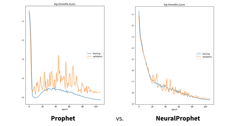
Prophet (2017) is the predecessor to NeuralProphet (2020) — the latter incorporates some autoregressive deep learning. Theoretically, NeuralProphet should always have equal or better performance than Prophet, so today we’re going to put that claim to the test.
Let’s dive in.
The Ground Rules
The Data
We’re going to be using a daily time series of California’s energy demand (figure 2).
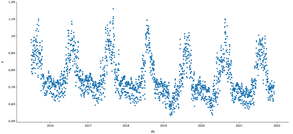
As you can see above, there is very strong yearly seasonality with peaks in the summers, probably due to increased air conditioning use. While less apparent from this chart, we’d also expect to see weekly seasonality — our hypothesis is that electricity consumption would differ between the weekend and weekdays.
With a traditional time series model like ARIMA, all this seasonality would require us to specify orders (look back indices) that corresponds to whatever level of seasonality we observe. The prophet models, on the other hand, automatically encapsulate this sinusoidal motion with Fourier Series’, so both Prophet models should effectively leverage the above seasonality.
Finally, taking one more observation about the data, you’ll notice that the axis names are y and ds. We’ve stored our time series in a pandas DataFrame that’s been restructured to fit Prophet’s specifications. The exact code that was used is the following…
df = read_data() # helper func
df = df[['Local date','D']]
df.columns = ['ds','y']
If you want to follow along, the data were downloaded from the source: U.S. Energy Information Administration (December 2021) and are available here as well. Here’s the copyright info.
Evaluation
Our metric of interest will be RMSE (figure 3).

To fairly compare our two models, we will leverage cross validation (CV). Note that traditional CV assumes that our data are exchangeable i.e. any ordering of our sample is equally likely to occur. With time series data, there’s a temporal component so unfortunately full randomization cannot be applied.
Instead, we try many different date cutoffs, training on all prior data and testing with the next n periods. This is called a rolling origin backtest. By iteratively training and determining out-of-sample accuracy, we can derive a more robust estimate of model accuracy.
In our case, we start our iterations at 2017–12–22 and, in increments of 180 days, end near 2021–12–06.
Competitor 1: Prophet
Our first competitor is Facebook Prophet. It is an open-source algorithm that has seen tremendous popularity since its inception in 2017. It’s main selling points are that it’s easy to use, interpretable, and easily interacts with a subject matter expert.
With introductions out of the way, let’s get coding.
First we are going to create our model and fit our restructured data.
m = Prophet()
m.fit(df)
Pretty complex, right? Next we’re going to develop a forecast and derive some key plots.
# create forecast
future = m.make_future_dataframe(periods=365)
forecast = m.predict(future)
# create plots
pred_plot = plot_plotly(m, forecast)
comp_plot = plot_components_plotly(m, forecast)
First, we create a data frame that is 365 periods into the future, in our case, 365 days. We then forecast accordingly and store predicted values along with prediction intervals in the variable, forecast. Finally, we create a prediction plot and component plot. Let’s take a look at each one in turn.
First we have our prediction plot in figure 4.
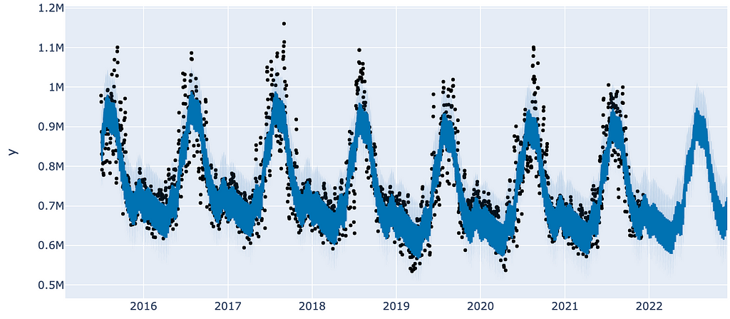
As you can see around 2022, our data stop and our forecast begins, as indicated by the lack of observations (black dots).
Ok this is a pretty picture, but it doesn’t tell us a ton about what’s going on behind the scenes. For that we’ll turn to a component plot (figure 5).
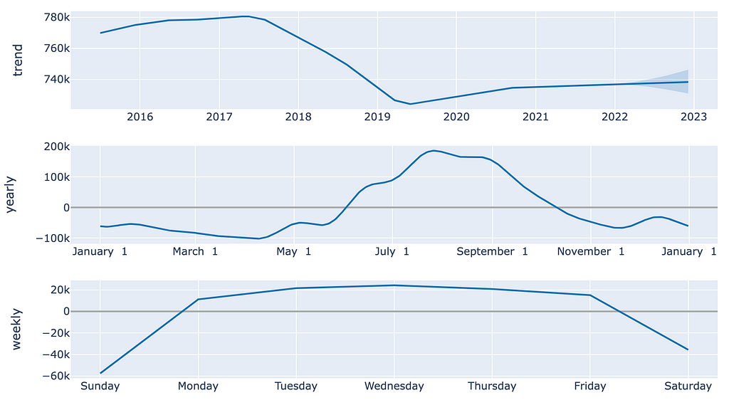
In the above plot, we have three charts, all of which provide useful conclusions about our data. First, we can see that in our top plot, trend is pretty unstable throughout the duration of our data. Starting in the middle of 2017, we saw a decrease in electricity demand, but the overall magnitude of the drop isn’t enormous. Second, according to the second chart, electricity demand is highest during the summer months and lowest in spring. These observations are consistent with our intuitions. Third, it seems that consumption on the weekends is significantly lower than on the week days. Again, this aligns with our expectations.
Talk about an interpretable model!
Prophet’s component plots are a tremendously useful window into what’s going on behind the scenes — no more black boxes. And note that NeuralProphet has the same functionality.
But, a model is only as good as its accuracy, so let’s take a look at accuracy.
Using the built in cross validation methods, the RMSE observed for a 365 forecast is 48810.12. Our y value is in the hundreds of thousands, somewhere between 600k and 1.2M, so an RMSE of 48k seems to be pretty low.
Let’s see if we can beat this with some deep learning.
Competitor 2: NeuralProphet
Our next model is the second iteration of Prophet. It incorporates deep learning terms to our equation which are fit on autoregressed (lagged) data. Theoretically and empirically, NeuralProphet is a superior model. But let’s see if this superiority holds for our energy demand dataset.
Let’s get coding.
First, as with Prophet, we need to create and fit a model. And note that syntax is very similar between the two iterations of Prophet.
m = NeuralProphet()
metrics = m.fit(df, freq="D")
Now that we’ve created our model, let’s create a forecast and get some key plots. We will be using the default parameters in NeuralProphet, which do not incorporate deep learning.
# create forecast
df_future = m.make_future_dataframe(df, periods=365)
forecast = m.predict(df_future)
# create plots
fig_forecast = m.plot(forecast)
fig_components = m.plot_components(forecast)
fig_model = m.plot_parameters()
As in the values above, let’s take a look at our forecast plot (figure 6).
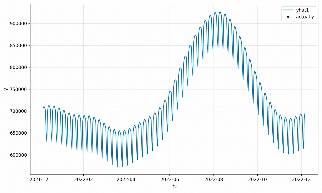
The values shown above are zoomed in much more than the prior forecast, but both have the same structure. Overall, they seem to have nearly identical values as well, which is expected because they’re both using Prophet without deep learning.
Finally, the built-in accuracy measure using default parameters for NeuralProphet is an RMSE of 62162.133594. After some digging, it turns out that the two libraries use different backtesting functions, so we will create a custom function that allows for a fair comparison. And, we’ll break out the deep learning.
The Verdict
Ok now that we have a feel for both libraries, let’s execute our competition.
First, we define our custom rolling backtest function. The key concept is that we create many train/test splits, as shown below.
train_test_split_indices = list(range(365*2, len(df.index) - 365, 180))
train_test_splits = [(df.iloc[:i, :], df.iloc[i:(i+365), :])
                     for i in train_test_split_indices]
From here, we can iterate over train_test_splits, train both models, and compare the results.
With our data set up, we are ready to break out the deep learning in NeuralProphet…
neural_params =  dict(
    n_forecasts=365,
    n_lags=30,
    yearly_seasonality=True,
    weekly_seasonality=True,
    daily_seasonality=True,
    batch_size=64,
    epochs=200,
    learning_rate=0.03
)
As shown above, we have activated the autoregression functionality through the n_lags parameter. We’ve also added some other potentially useful parameters, such as setting the number of epochs, seasonality types, and the learning rate. And finally, we’ve set our forecasting horizon to be 365 days.
After running both models through our rolling origin backtest, we get the following RMSE’s. Note that we also included Mean Absolute Percent Error (MAPE) for interpretation purposes.
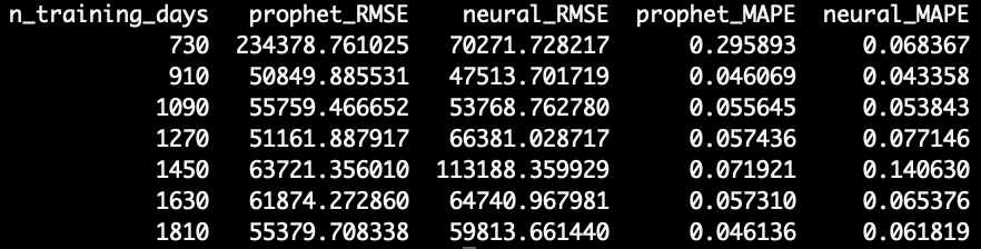
The results are pretty surprising.
When trained on 730 days, NeuralProphet far out-performs Prophet. However, with 910 and 1090 days of training data, NeuralProphet beats Prophet by a slim margin. And finally, with 1270 days or more of training data, Prophet surpasses NeuralProphet in accuracy.
Here, NeuralProphet is better on smaller datasets, but Prophet is better with lots of training data.
Now we wouldn’t expect this outcome prior to running the models, but retrospectively, this sort of makes sense. One reason deep learning methods are so effective is they can fit extremely complex data. However, if too much noisy data is provided, they can overfit which makes simpler and “smoother” models perform better.
One possible explanation is that with enough training data, Prophet is more effective on very cyclical data. If the majority of the motion is sinusoidal due to seasonality (which appears to be the case), it will be hard to improve upon a Fourier-Series-based model.
If you’re curious to reproduce the results, check out the code here. Also, if there is incorrect implementation, please leave a comment here or on the repo.
Prophet vs. The Government
Finally, we’re going to end on a fun note.
Each day the EIA publishes a day-ahead forecast. Curious to see how our annual models compared, I quickly calculated the RMSE and MAPE for the government’s forecast. The values were 28432.85 and 0.0242 respectively.
Comparing these numbers with the numbers in the above table, our Prophet models has roughly double the error, but for a 365 day forecast horizon. The government is looking just one day ahead.
A cool and easy follow up would be to try to beat the government using either Prophet model. Shouldn’t be too hard, right?
Thanks for reading! I’ll be writing 24 more posts that bring academic research to the DS industry. Check out my comment for links to the main source for this post and some useful resources.
Prophet vs. NeuralProphet was originally published in Towards Data Science on Medium, where people are continuing the conversation by highlighting and responding to this story.
from Towards Data Science - Medium https://ift.tt/3FbKcCw
via RiYo Analytics


ليست هناك تعليقات