https://ift.tt/3sNPn8K Neural Networks and Neural Autoencoders as Dimensional Reduction Tools: Knime and Python Implemented with Knime and...
Neural Networks and Neural Autoencoders as Dimensional Reduction Tools: Knime and Python
Implemented with Knime and Tensor Flow in Python, analysing data in the middle of the diabolo.

In my first story I wrote a humble story about embedding images from the MNIST dataset from OpenML, of handwritten numbers from 0 to 9, by Yann LeCun, Corinna Cortes and Christopher J.C. Burges. I used the UMAP algorithm for dimensional reduction. After that, I used DBSCAN for clustering and identify the original clusters. I will use again the same dataset.
What is the proposal of this story?
Now I will explore quite a similar path but I will use a Neural Network and a Neural Autoencoder, instead of the UMAP algorithm, for dimensional reduction. I will do that both within Knime, with Keras integration, environment and with TensorFlow in Python. After dimensional reduction, I will use DBSCAN to verify whether the clusters created by the neural networks can be identified…, or not. All codes and workflows will be shared.
For more information about codeless deep learning I suggest the following book of Rosaria Silipo and Kathrin Melcher: “Codeless Deep Learning” as a guide for a quiet walk through deep learning within Knime environment.
Neural Autoencoders
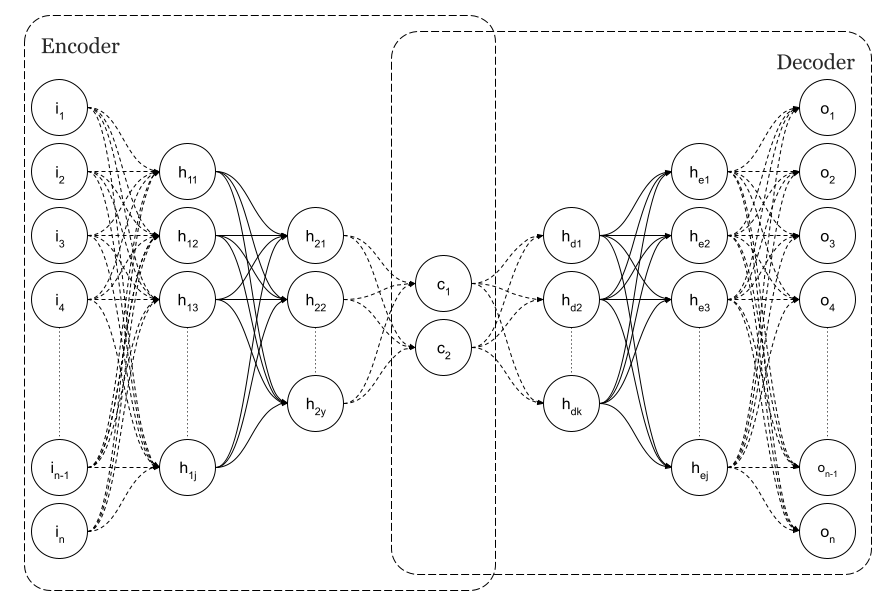
Simple Neural Autoencoders are a particular architecture of feedforward neural networks in which, as can be seen in previous Figure 1, the dimension of the input layer is equal to the dimension of the output, n as per image.
Autoencoders are trained, as regular feedforward neural networks, by means of back propagation, in order to get an output equal to the input. As a result, they are capable of reproducing the inputs they have been trained with. As a matter of fact, if we feed the trained network with an input similar to those that were use during training, the expected output is to be very close to the input. If that did not happened, we could conclude that the input was not a “regular” or common input. That capability is often used to detect, for instance, fraudulent credit card transactions. Since not many fraudulent card transaction data is available, it makes sense to train the network with normal transactions data and if, eventually, the network is not able reproduce the input we could say we are facing a fraud. That is why Autoencoders are considered an unsupervised algorithm. You can find more information about autoencoders on the following articles of TDS, Anomaly Detection using Autoencoders or Applied Deep Learning — Part 3: Autoencoders and you can also check my public list of Autoencoders stories.
Going back to my original purpose which was using autoencoders as dimensional reduction technique, as you can see in Figure 1, there is a layer of minimum dimension. The centre of the diabolo.

Particularly in the figure, dimension is n=2. That layer is the code. It is called the latent space. At that point in the neural network, we can consider that we have codified the input and we should be able to detect, in this case in a 2D graph, that we have different clusters of points according to the different implicit classes existing in the input data.
Structure and Sources
We will perform that test in Knime and in Python using TensorFlow.
Some configurations will be needed in Knime so you can train a neural network with Keras. Please, follow this tutorial KNIME Deep Learning — Keras Integration.
This article is structured as follows:
Part 1. Dimensional reduction with Autoencoders
As described above, we use simple dense autoencoders for dimensional reduction and will compare its implementation in Knime and Python step by step.
Part 2. Dimensional reduction with Dense Neural Networks
Another interesting approach will be performed. Since the reference dataset for this tests has information about the class of each sample, instead of using an autoencoder, a dense neural network will be used with an internal layer of 2 or 3 neurons so a sort of latent space will be defined. Please check the following Figure 3 describing the network with a particularised number of classes C=10 which is the case of our dataset.
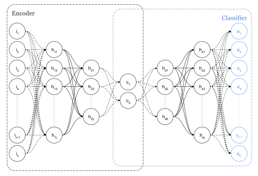
Similarly, we will analyse this implementation in Knime and Python step by step.
Before we begin, you will find all Python codes in my GitHub and the Knime workflows in my public space within the Knime Hub.
Knime workflows
You will find Knime Workflow containing two different solutions for each of the different approaches:
Part 1. Dimensional reduction with Autoencoders. The workflow will diverge in two different endings for 2D and 3D latent spaces. Alternatively,
Part 2. Dimensional reduction with Dense Neural Networks has also two different branches for 2D and 3D minimum dimension representation.
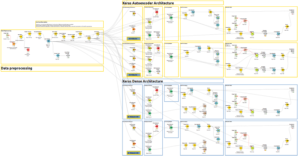
Let me show you a global overview of the whole workflow so you can understand the different branches.
In Figure 3bis, yellow workflows correspond to autoencoder architecture in Part 1 for 2D and 3D and, alternatively, blue workflow corresponds to Part 2 for dense architecture.
Python codes
Two Python codes are available:
KNIME_Replication_3D_Midpoint.py performing training and inference with an Autoencoder and KNIME_Replication_3D_Midpoint_DM.py performing training and inference with a dense connected network. In both codes, when the code is executed with no arguments, a latent space of 3D is assumed. However, you can pass an argument indicating the desired size of the latent space, for instance 3.
pyhton3 KNIME_Replication_3DMidpoint_DM.py 3
An auxiliary Python file is also provided, ml_functions.py, within which, a class ModelGr and its methods are defined and used in main codes.
Part 1. Dimensional reduction with Autoencoders
Data Preprocessing
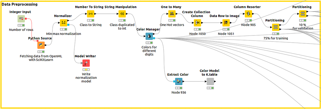
As shown in Figure 4, we capture the data with a Python Source Node, we normalise the data and, immediately after that, we use the Color Manager node to define a color code that will be assigned uniquely to the class all over the workflow so different plots will have the same legend. After that, different partitions for training and validations are built.
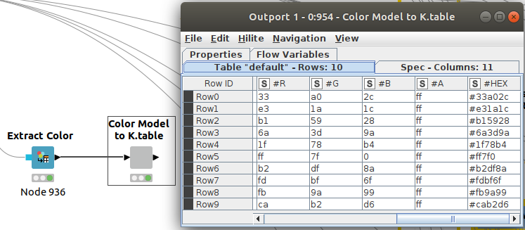
With previous nodes in Figure 5, we can extract the color codes (in column #HEX) we are using so we can reuse them in Python. That will make it easier to compare results.
Part of the initial Python code, related with fetching the data and partitioning, follows in Code 1.
Normalization is done whenever forward inferences are performed with the forward method defined for the class ModelGr(). See following Code 2, Line 5.
Keras Neural Network Architecture
The neural architecture is defined in Knime as a sequence of Keras Dense Layer nodes. Following, in Figure 6, a global scheme of the definition is shown.
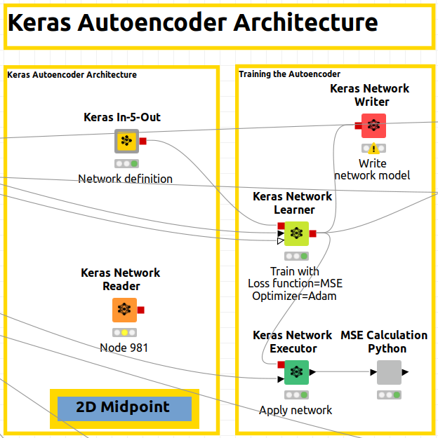
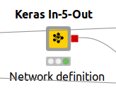
There is a special node shown in Figure 7. That is a component node which encapsulates several nodes and a configuration interface with functional parameters defining the performance of the inner nodes. In Figure 8, the sequence of layers is shown and, in Figure 9, you can find the parameters than can be configured for the componente. CTRL+double clicking in Network Definition component will enter in the inner node definition shown in Figure 8. Double clicking in in network definition component will open configuration window of Figure 9. Basically, layers sizes and activation functions can be defined.

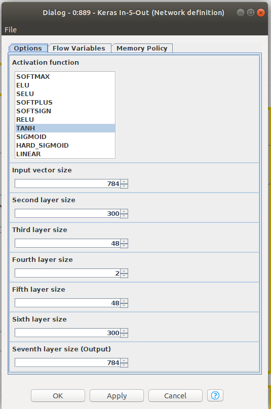
Please note that we have defined an input layer, five internal layers and the output layer. Activation function, at this point, is common for all layers, Hyperbolic Tangent, as per image in Figure 9. Layer configuration parameters, beyond above mentioned, can be configured entering the configuration of each node in Figure 8, that is to say, kernel and bias initializers, regularizers and constraints. Please note in Figure 9 that in the fourth layer we define the size as 2 for the case of a 2D latent space. For a 3D option, you will find an alternative workflow.
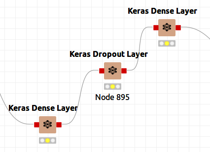
Although I did not use dropout layers to prevent overfitting, it would be so easy as can be seen in Figure 9bis. Just adding a Dropout layer and reconnecting the nodes.
For Python network a class ModelGr() has been defined and, when called, will be informed with activation functions, layer sizes, number of layers and name. See here the model definition in Code 3, Line 14+:
Conceptually, a sequential network is defined (Code 4, Line 15) and we recursively add layers with the size and activation functions included in the call (Code 4, Lines 17+)
As can be seen in different Figures and codes, the networks have the following layers and sizes:
- [784 (input), 300, 48, 2 or 3 (latent space), 48, 300, 784] and
- the activation functions is hyperbolic tangent.
Training the network
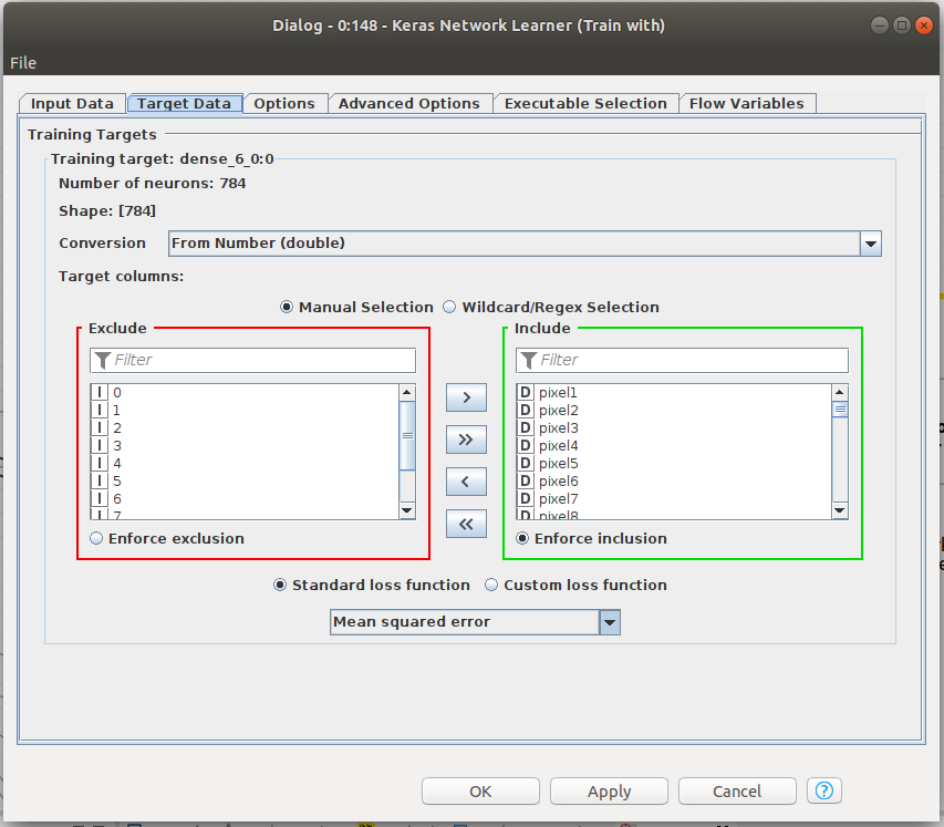
Training the network in Knime is easy. In previous Figure 6, the Keras Network learner just has to be fed with training data and validation data. The input and target data for the training has to be defined. Since we are training an autoencoder, input and target data have the same size, particularly, the 784 pixels of the images from MNIST. The loss function to be minimized in the training is defined in that node, among other parameters. Please note that we are choosing MSE, Mean squared error. We will train to minimize MSE between the input and the output vectors since, ideally, we want them to be equal.
For Python and TensorFlow, a training function has been defined. Please note ,in Code 5 Line 21, the definition of the loss function as a RMSE, Root Mean Squeare Error, as we did in Knime. RMSE_loss() method is defined in the class ModelGr() and can be found in Code 5bis.
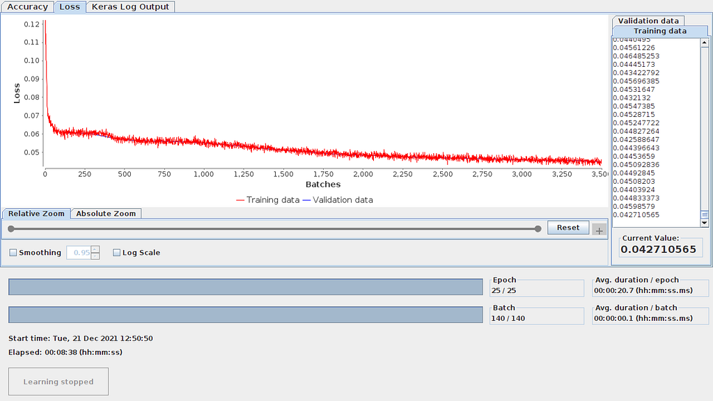
Should you need to check how the training evolved, that can be done in both approaches. In Knime, in the Keras Network Learner node, right click and click on “View Learning Monitor”. See learning monitor un Figure 10.1
In the case of TensorFlow, TensorBoard can be used to collect and analyze the network.
TensorBoard provides the visualization and tooling needed for machine learning experimentation:
-Tracking and visualizing metrics such as loss and accuracy
-Visualizing the model graph (ops and layers)
-Viewing histograms of weights, biases, or other tensors as they change over time
-Projecting embeddings to a lower dimensional space…
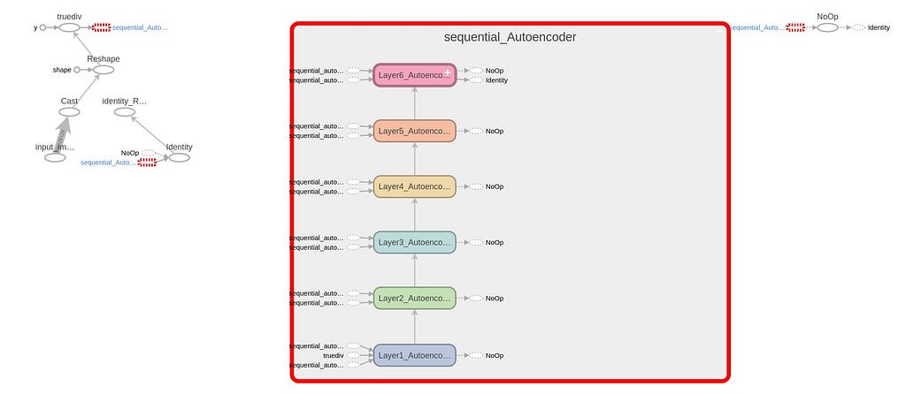
In Code 5, several code lines are added (6,22,23,30+) to gather data about training and network graph, weights and loss. The shared Python codes, both dense and autoencoder, launch automatically TensorBoard before ending execution. In Figures 10.2 and 10.3 you can see the graph and the loss evolution.

Extracting the midpoint
We have trained the networks, which are configured as Neural Autoencoders and now it is time to get the output. In Knime, please note in Figure 11, that the Keras Network Learner has a red output port. That output is the trained network model. So executing the network is just connecting the Keras Network Executor node informed with the model and the data. But care must be taken.
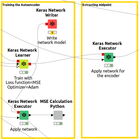
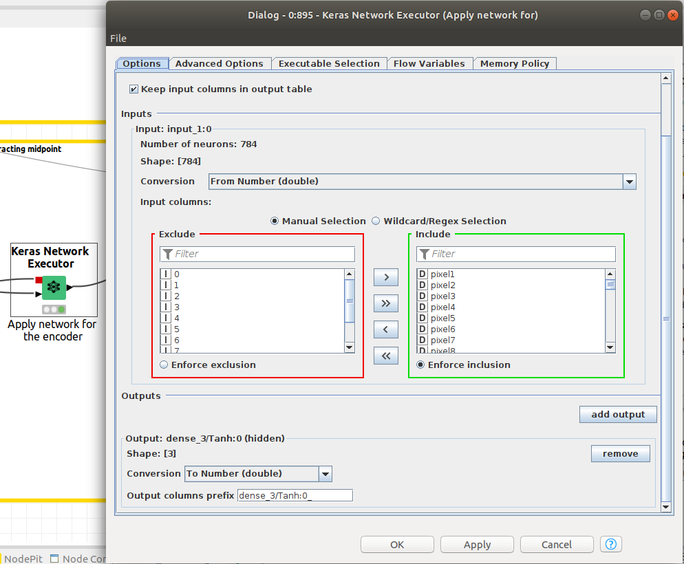
Remember that we want to extract the latent space of the autoencoder so we have to configure the Keras Network Executor node to offer that paticular output. That is done by defining the layer corresponding to the latent space as an output. Figure 12 is showing how to configure latent space as the output of the Network Executor node.
In Python, we had built a compact sequential network and, to extract the midpoint, we use a class named Encoder(). When defining an object as Encoder() ,by calling Encoder = mli.Encoder(model) and being model a sequential network model, the __init__ method will extract the layers of the network and will add them to another sequential network from the initial layers to the minimum sized layer, that is to say, the latent space. See condition in Code 6, Line 9.
A forward method is defined for inferring the Encoder. It is shown in Code 7.
Encoder has been defined as the portion of the neural network from the initial layer to the minimum sized layer so the forward method will deliver the latent space.
Results for autoencoders networks
Graphical results for latent space will be shown.
2D Results and attempt to get clusters.
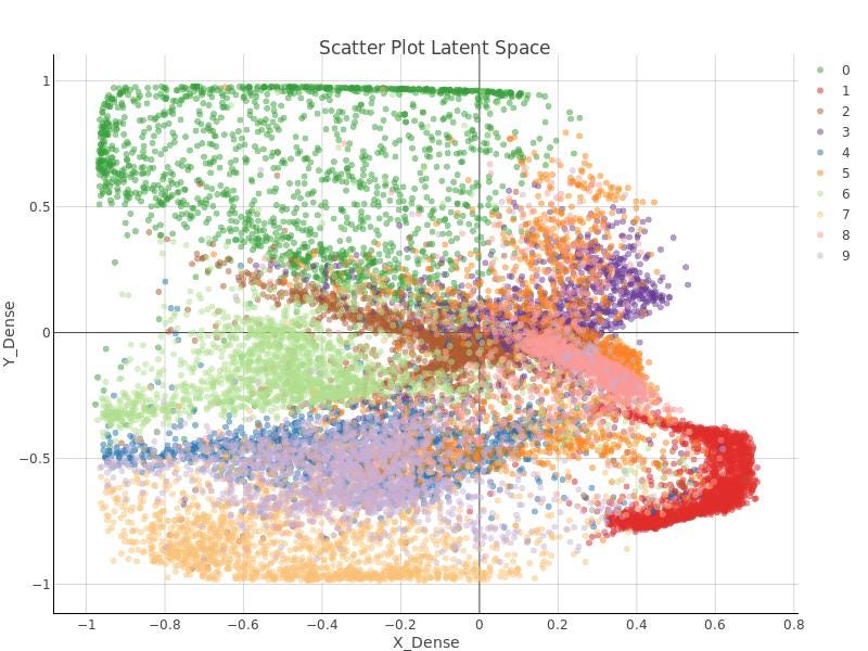
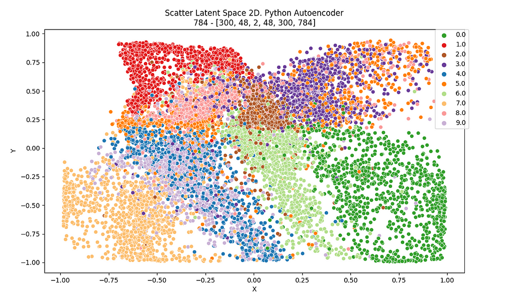
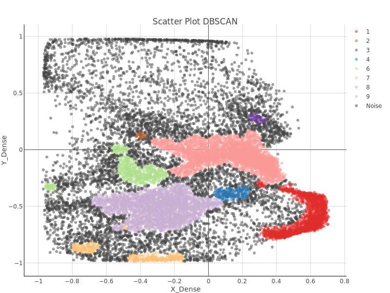
In Figure 12 and 13, the 2D latent space of the autoencoder is plotted for both environments, Knime and Python. It can be checked that some sort of order and coherence can be perceived by human eye but, applying DBSCAN algorithm on that data won’t lead to any cluster related to those that were defined in the latent space of the autoencoder.
In the righter part of the autoencoder workflows, DBSCAN algorithm is applied. Remember DBSCAN is ruled by two parameters:
epsilon: Specifies distance between points so they can be be considered a part of a cluster. Two points will be considered neighbors belonging to the same cluster if the distance between them is lower than epsilon.
minimum points: Minimum number of points reachable from a point p so that p point can be considered a core point.
After a few tests, no pair of those parameters was found to get the right clusters. In Figure 15, just to leave testimony of such attempts, DBSCAN clusters are shown.
3D Results and attempt to get clusters
Alternatively, I carried out the same work but with a 3D latent space. Not too much changes to be explained but the fact that the dimension of the layer defining the latent space both in Knime and in Python is, logically, 3 instead of 2.
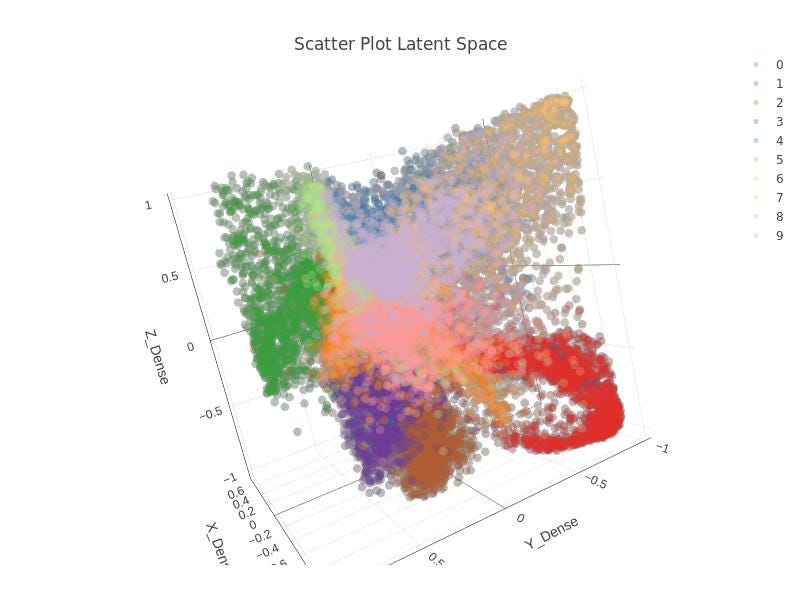
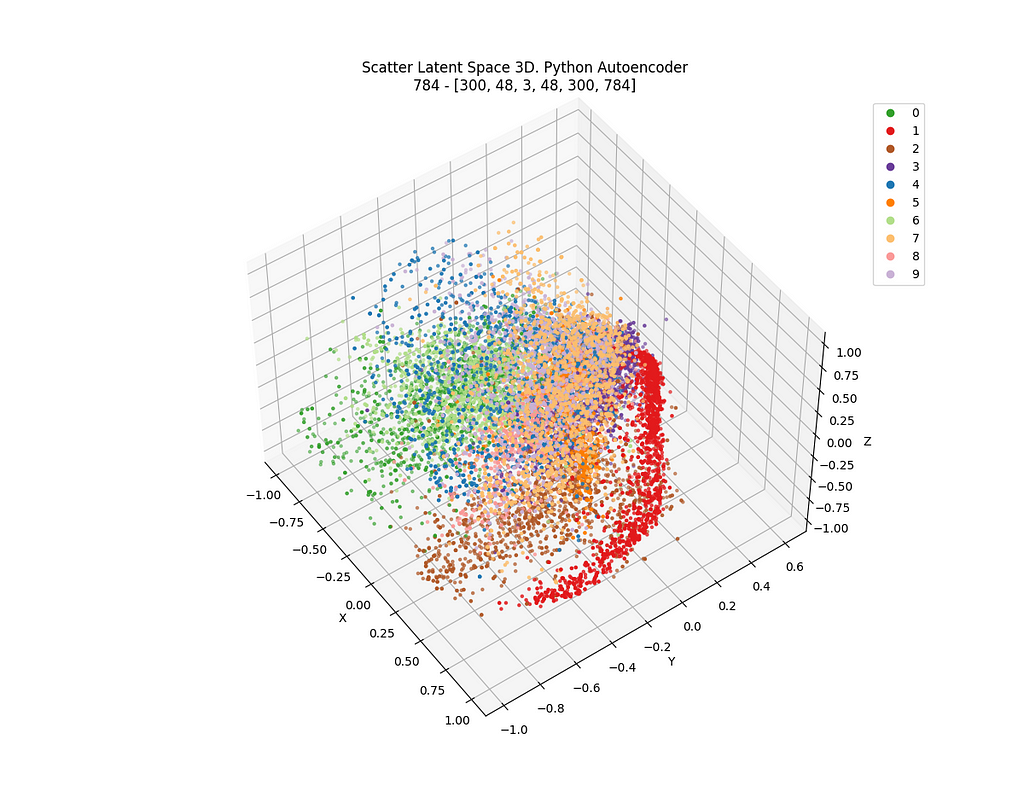
See in the following images in Figure 16–18, from Knime and Python for the latent space in 3D.
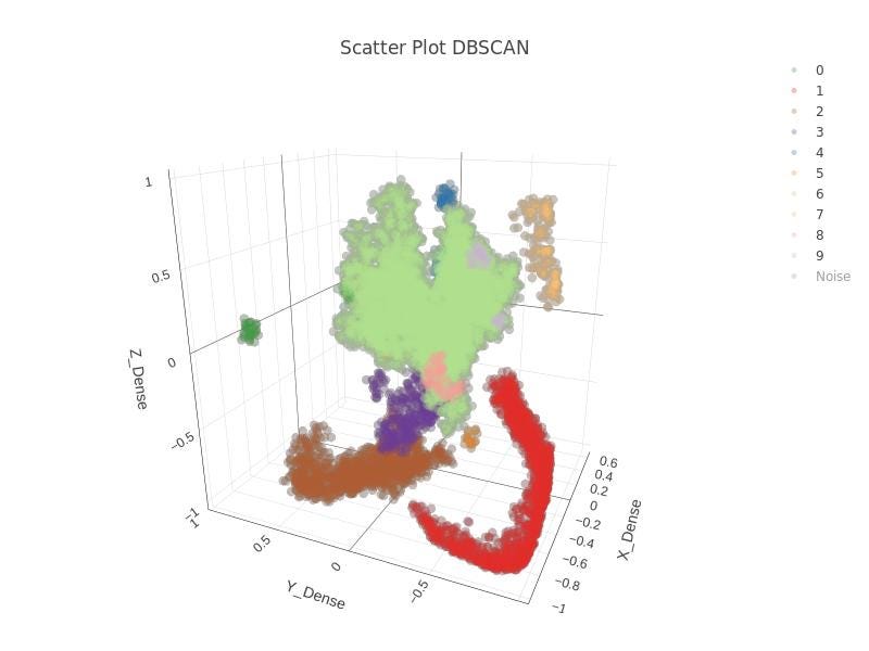
It can be checked, again, that some sort of order and coherence can be envisaged, but, again, applying DBSCAN algorithm on that data won’t lead to any similar cluster related to those that were defined in the latent space of the autoencoder. Check Figure 18.
Images resulting from autoencoder
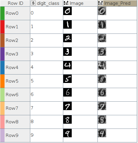
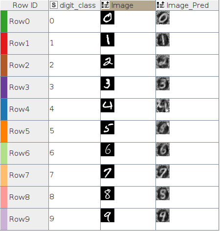
In Figures 18.1 and 18.2 you can find the best and worst images according to the MSE calculations after inference for the 3D latent space autoencoder.
Part 2. Dimensional reduction with Dense Neural Networks
Well, so we could say that, so far, this is the story of a defeat.
I tried another approach before surrender. As I explained, since we have the class of each sample in the dataset, a network like the one in Figure 3 can be conceived both for a latent space of 2D and 3D. That is a classifier network with a minimum sized, 2 or 3, internal layer that could be considered as the latent space.
Differences
Obviously, there is a major change in the loss function for the training. Now we want to optimise a classifier and a right loss function to do that, is the cross-entropy loss. Cross-entropy loss is mainly used in combination with Softmax activation function.
It is interesting to take a look into those concepts.
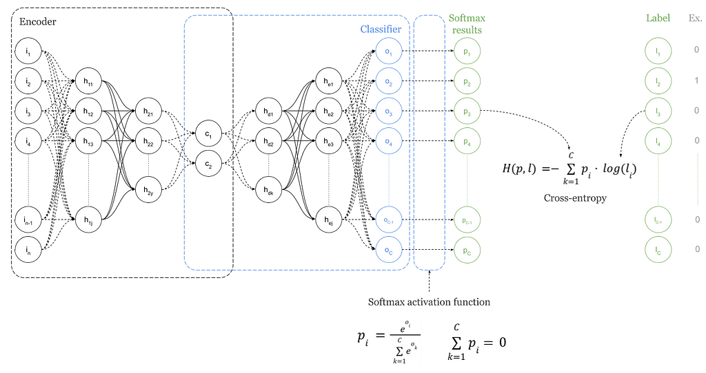
In the above Figure 19, Softmax converts logits, vector O, into probabilities, vector P. The purpose of the Cross-Entropy is to take the output probabilities contained in vector P and measure the distance from the class values expressed in the labels vector L as a One-Hot vector. See example vector on the right side of Figure 19.
The objective is to make the model output to be as close as possible to the desired output (class values). How do we do that?
Knime
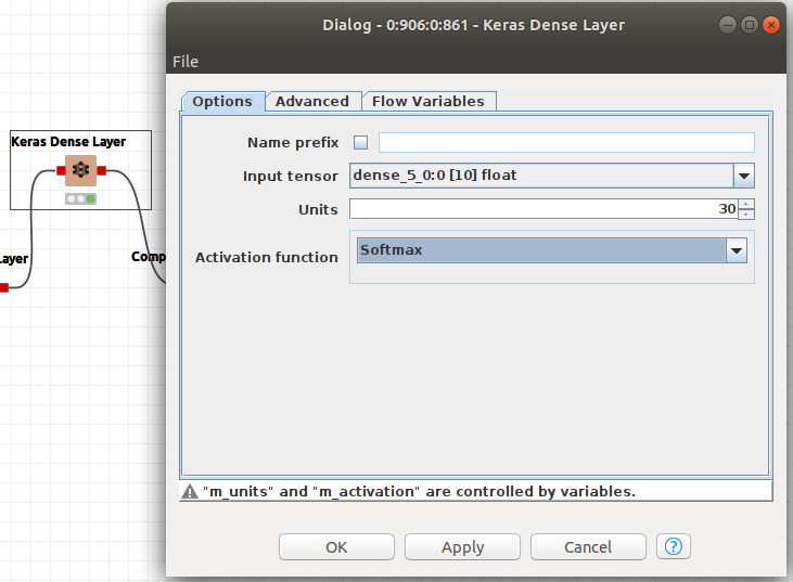
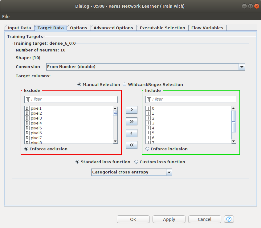
Softmax has to be defined as the activation function for the last Keras Dense Layer and the Cross-Entropy as the loss function in the Keras Network Learner. See Figures 20 and 21.
Python and Tensor Flow
As done before, a loss function has to be defined according to the exposed criteria. See Code 8.
Sparse Softmax cross entropy between logits and labels is performed in Code 8. Using sparse variation of Cross-Entropy function, there is no need to build a One-Hot vector and the labels can be fed directly.
The networks have the following layers and sizes in both platforms:
- [784 (input), 300, 100, 10, 2 or 3 (latent space), 10, 10] and
- the activation functions are hyperbolic tangent and softmax for the output layer
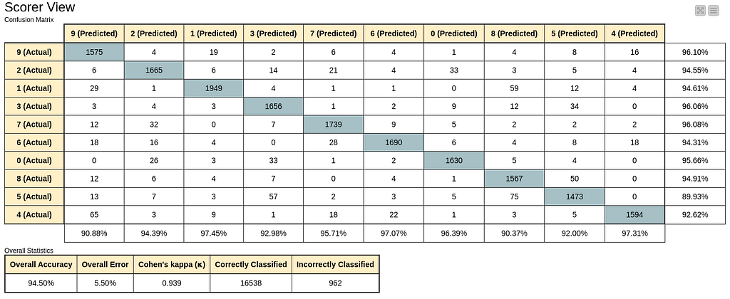
Overall accuracies for both platforms and for both 2D and 3D latent spaces are between 94% and 96% with confusion matrices similar to the following in Figure 23, extracted from the Scorer node in Knime, in Figure 22.
2D Results and attempt to get clusters.
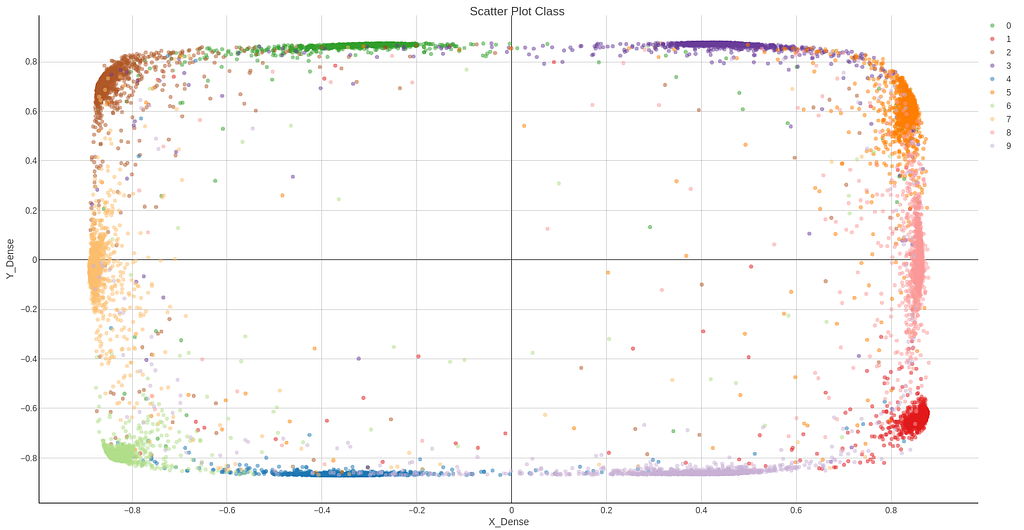
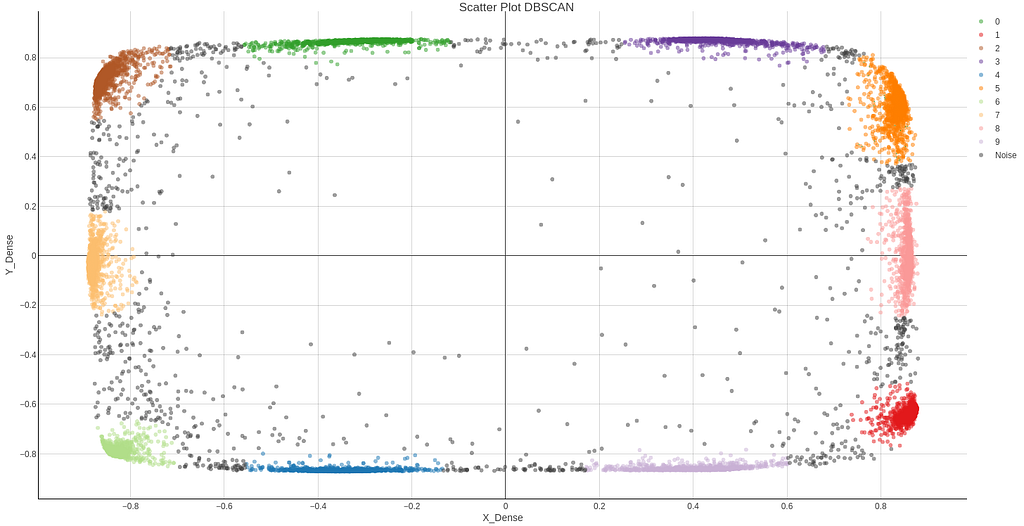
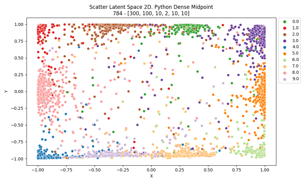
Following you can find the results for the 2D latent space of the new approach, both in Knime, Figure 24, and Python, Figure 26. Now clusters can clearly be distinguished and DBSCAN algorithm detects them easily. DBSCAN is performed on Knime results and is shown in Figure 25.
3D Results and attempt to get clusters.
No further explanations are required before taking a look in 3D results. For neural dense architecture I have prepared some nodes in Knime to prepare data to be imported in Plotly so you can explore and interact with the plot. Not a big job but that is also contained in the workflow so you may want to explore it and reuse it.
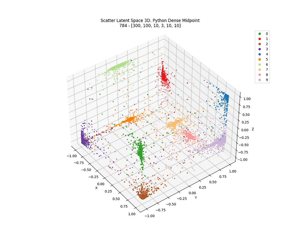
In Figure 27, the 3D latent space is shown and in Figure 28 you can find the DBSCAN clustering. Quite a nice result with this approach. Clusters are identified. By clicking in the legends, traces can be hidden.
And finally, the result of TensorFlow for dense network in 3D in Figure 29, which is static.
Conclusions
My purpose was to explore an idea, using neural networks for dimensional reduction, down to a dimension of 2 or 3 which is very restrictive, and do that in two environments, Knime and Python. In a rough approach it was not possible to extract clear clusters from a neural autoencoder with no further refinements in none of those environments. Latent spaces down to 2 or 3 dimension is a good option to explore graphically but it is too limited to capture the characteristics of the original object. On the other hand, it was possible indeed to do it with a dense neural classifier with an internal layer of dimension 2 or 3 in both environments. We can conclude that results in Knime with Keras Integration and Python with Tensor Flow can be considered equivalent, at least for the scope of this article. That, in my opinion, is good news, since there is a wide opened gate to machine learning without the need of strong and solid coding background and, hence, the more people that can contribute, the further we will all arrive together.
In the near future I will explore those necessary refinements in autoencoders so I can get my initial goal.
Neural Networks and Neural Autoencoders as dimensional reduction tools. Knime and Python. was originally published in Towards Data Science on Medium, where people are continuing the conversation by highlighting and responding to this story.
from Towards Data Science - Medium https://ift.tt/3pGn89M
via RiYo Analytics

No comments