https://ift.tt/3GbqJCa Identifying indoor Wi-Fi users’ locations with a tolerance of uncertainty by Pymc3 Wi-Fi sensor network With the...
Identifying indoor Wi-Fi users’ locations with a tolerance of uncertainty by Pymc3
With the help of GPS, outdoor positioning has witnessed significant development. However, we are suffering from important inaccuracies when facing the indoor case. The existence of Wi-Fi network gives an alternative to build a localization system and significant research has been done in this area in the past years, among which localization based on wireless signal strength information has attracted attention thanks to its low-cost and easy implementation. However, due to the difficulty to get location labels of the data, supervised models are sometimes difficult to build in practice.
In this article, you will be reading:
- An unsupervised model to learn Wi-Fi users’ location based on received signal strength indicator (RSSI).
- How to use the Bayesian model framework Pymc3 for localization with a tolerance of uncertainty.
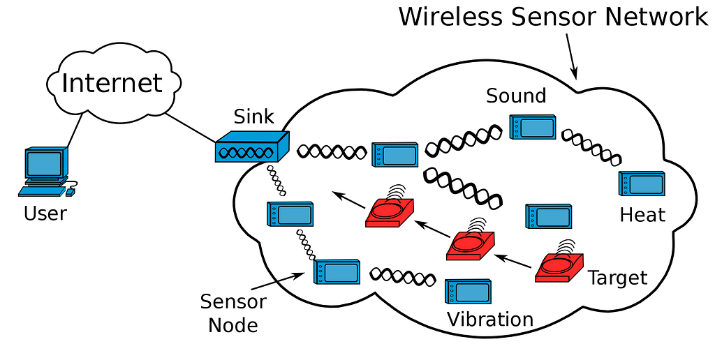
Wi-Fi users’ localization based on RSSI
RSSI localization techniques are based on measuring the RSSI value from a client device to several different access points and then combining this information with a propagation model to determine the distance between the client device and the access points. The value of RSSI can be captured by a wireless sensor using a type of short-range passive radar technology with surprising accuracy. In practice, unfortunately, it is hard to get a 1–to-1 pair of a device’s location and its value of RSSI received by a sensor at an access point. However, the good news is that in our case, despite the lack of labeled data, the physics behind can help us build an unsupervised model. For a device d and a sensor s at a certain access point, the following equation has been proved by physical experience:

where a is a constant and p(s), p(d) the positions of the sensor and the device. The three remaining functions’ values depend only on the device and the sensor.
From this equation, we can see that it is relatively simple to get the RSSI value once we know the value of the constant a the expressions of the three remaining functions and positions of the device and the sensor.
For the sake of simplicity, we suppose that all the three functions are constants, that is, the equation can be simplified as a linear regression of the log distance of the device and the sensor:

Suppose that you know the exact value of the constants in the above equation and where the sensor is, it is straightforward to identify a sphere on which the device is for the equation is satisfied. Theoretically, we only need 4 sensors to localize a device. But attention, the problem is more complicated than the theory for three main reasons:
- We don’t have any access to the two constants in the equation.
- The RSSI measurements tend to fluctuate a lot according to changes in the environment so that the equation does always not hold.
- We suffer from an important loss of data in practice.
Bayesian model for device localization
Imagine now we have a provided dataset of RSSI values from several sensors which might have a bad quality: loss of data of a part of sensors, weakened signals, etc. What can we do to localize the Wi-Fi users who sent these RSSI values from their devices? My suggestion is: give the model the right to have some uncertainty. This uncertainty is tolerated in many use cases: e.g. in a shopping mall, it suffices that the operator knows in which shop/zone a user is instead of an accurate point.
Assume that we know the positions of all Wi-Fi sensors. The target space is discretized into locations. The unknown constants follow some normal distributions. The idea of the model is to first assume that the target could be these locations with some probabilities and these probabilities can generate a distribution of RSSI values. Now for a given RSSI vector, the goal is to find a position and a pair of constants that could generate this given vector, that is, to maximize the likelihood log(p(RSSI|d; a,c)).
Recall that we said in the last section that The RSSI measurements tend to fluctuate a lot according to changes in the environment. We thus make one more assumption here that the value of RSSI of a given sensor and sent by a given device follows a normal distribution.
Modelling with Pymc3
Now let us see how to build the model with Pymc3: a nice tool for Bayesian statistical modeling and probabilistic machine learning. One thing more to emphasize is that Pymc3 will just skip the lost RSSI values (Nan) in training: imagine that you have 8 sensors have 2 of them have lost the RSSI values of one device and Pymc3 will train the model with the 6 remaining ones.
Let us first import all the packages we need:
import pymc3 as pm
import theano.tensor as tt
import numpy as np
import pandas as pd
from statistics import median
Now let us build a Wi-Fi localization model whose inputs are: 1. bounds: the boundaries of target spaces in which we do sampling; 2. observations_n: the total number of observed RSSI values; 3. rssis: the provided RSSI values; 4. sensor_positions: the positions of sensors; 5. sensors_n: the total number of sensors. In the code below, I simply did two things:
- Sampling parameters and target locations with prior distributions.
- Build a pm.model as a normal distribution.
def wifi_localization_model(
    bounds,
    observations_n,
    rssis,
    sensor_positions,
    sensors_n,
):
rssis=pd.DataFrame(rssis)
    dimensions_n = len(bounds)
    #build the pm model
    model = pm.Model()
    sensor_positions=sensor_positions.reshape((1, sensors_n, dimensions_n))
    with model:
        device_location_dimensions = []
        device_location_variables = []
        #sampling the positions of the devices with a normal distribution
        for i, bound in enumerate(bounds):
            x = pm.Normal(
                name="x_{}".format(i),
                mu=(bound[0] + bound[1]) / 2,
                sigma=(bound[1] - bound[0])/4 ,
                shape=len(rssis),
            )
            device_location_variables.append(x)
            device_location_dimensions.append(tt.reshape(x, (-1, 1)))
        device_location = tt.concatenate(device_location_dimensions, axis=1)
        device_location = tt.repeat(
            tt.reshape(device_location, (len(rssis), 1, dimensions_n)),
            sensors_n,
            axis=1,
        )
        #sampling the constants of the RSSI equation with a uniform distribution
        n_var = pm.Uniform(name="n", lower=0, upper=10)
        gain_var = pm.Uniform(name="gain", lower=-100, upper=-20)
#sampling the noise of the RSSI with a normal distribution
        noise_std_var = pm.Uniform(name="noise_std", lower=0, upper=100)
        log_distance = (
            -10
            * n_var
            * 0.5
            * tt.log10(
                tt.sum(
                    tt.sqr(
                        device_location
                        - np.repeat(sensor_positions, len(rssis), 0)
                    ),
                    axis=2,
                )
            )
        )
        rssi = log_distance + gain_var
        pm.Normal(
            name='observation', mu=rssi, sigma=noise_std_var, observed=rssis
        )
        # start with the initializer "advi"
        tr = pm.sample(
            draws=3000,
            tune=500+dimensions_n * 100,
            chains=4,
            init="advi",
            target_accept=0.75 + 0.05 * dimensions_n,
        )
        n= median(tr['n'])
        gain=median(tr['gain'])
        noise=median(tr['noise_std'])
        estimated_location = []
        estimated_std = []
        locations = []
        for i, device_location_variable in enumerate(device_location_variables):
            summary = pm.summary(
                tr, var_names=[device_location_variable.name]
            )
            estimated_location.append(
                summary["mean"].values.reshape(-1, 1)
            )
            estimated_std.append(summary["sd"].values.reshape(-1, 1))
estimated_std.append(summary["sd"].values.reshape(-1, 1))        predictions = np.hstack(estimated_location)
        estimated_std.append(summary["sd"].values.reshape(-1, 1))
estimated_std = np.hstack(estimated_std)
return (
            predictions,
            estimated_std,
            gain,
            noise,
        )
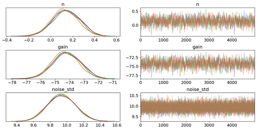
Results
I have tested the model on a synthetic dataset that I generated myself with 21 sensors. Of course, I removed a part of the data to simulate the case of data loss. Here is the trace plot of all the constants in the RSSI equation:
Here is a comparison of the Bayesian model’s error from that of a normal random guess and a uniform random guess:
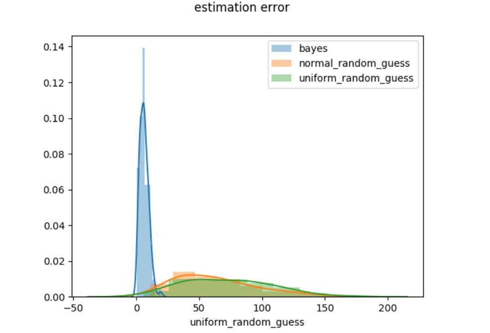
We have achieved good accuracy!
Before concluding this article, I want to show you an experiment that I did in my place: I installed 6 Wi-Fi sensors and fit the model with the RSSI values I got from them. With the estimated_mean and estimated_std, I can draw a sphere inside which a device can be at every moment. Furthermore, by giving such predicted spheres every 5 minutes, I can draw the trajectory of a Wi-Fi user that interests me. The Gif below was my trajectory during one hour:
Conclusion
In this article, we build a Bayesian unsupervised model to localize indoor Wi-Fi devices based on RSSI data with a tolerance of uncertainty. With the help of probabilistic programming provided by Pymc3, we have achieved good accuracy despite the imperfect quality of the data with relatively easy implementation.
Localization of indoor Wi-Fi users by Bayesian statistical modelling was originally published in Towards Data Science on Medium, where people are continuing the conversation by highlighting and responding to this story.
from Towards Data Science - Medium https://ift.tt/3Dp6san
via RiYo Analytics


ليست هناك تعليقات